


This article is a sequel to our earlier one on using SQL for data analysis. In case they’ve missed it, readers are advised to read the earlier article published in the February 2020 issue of OSFY.
Comparing different parameters of a data set is a common practice to derive a meaningful conclusion. The sample data may be something like rainfall vs agricultural production, stock-index vs GDP or other such data from business and academic fields. Different prediction techniques are used for these studies to estimate their relationships. Nowadays, plenty of ready-to-use computational solutions are available and due to the easy availability of IT infrastructure, even those without tech degrees are using these tools for their own benefit.
To identify the relationship between two or more related features, correlation and regression analyses are commonly used. Regression analysis explores the existence of any linear relationship while correlation establishes the strength of that linear relationship. A linear regression is a statistical model that analyses the relationship between a response variable (often called y) and one or more predictor variables and their interactions (often called x or explanatory variables). This technique is effective and easily understandable unlike other data analysis algorithms like artificial neural networks, decision trees or random forests.
Basic descriptive statistics
To have a simple discussion on basic statistics, let us consider a customer table, containing the customer ID, age, income and average spending patterns. Using SQL, it is easy to get basic statistical values like the mean, median and mode of the different parameters of the customer table.
Average: Basic statistical parameters like the mean, median and mode can be computed using SQL functions either with built-in functions or from derived queries. For instance, to get the average age and the corresponding average income of the customer, one can use the following query:
select round(avg(Age),2) as Age_bar, round(avg(Annualincome),2) as Income_bar
from customer
| Age_bar | Income_bar |
| 38.95 | 60.79 |
Similarly, it is also possible to get the maximum and minimum ages as well as their corresponding income values. Median and mode features are not available in SQL and can be derived from other queries. In the earlier article, I have described the methods in detail.
Frequency distribution: Preparing the frequency table is an essential part of descriptive statistics and is also used for histogram plotting. It can be implemented simply by the count() function and the GROUP BY clause. To demonstrate its use, I have taken the ‘order detail’ table of the Northwind database to show the frequency of different products in the TABLE. The corresponding SQL statement is as follows:
USE northwind;
SELECT ProductID,COUNT(ProductID) AS Product-Frequency
FROM `order details` AS a
GROUP BY ProductID;
| ProductID | Product_ frequency |
| 1 | 38 |
| 2 | 44 |
| 3 | 12 |
| 4 | 20 |
| … | …. |
A little improvement in the above query can provide the percentage of the product count along with the frequency values. To do so, we require a sub-query to count the number of records for each category of ProductID. The query may be written as follows:
SELECT ProductID,
COUNT(ProductID) AS Product_Frequency,
ROUND(COUNT(ProductID)*100/(select COUNT(*) from `order details`),2) AS Percentage
FROM `order details` AS a
GROUP BY ProductID;
| ProductID | Product_Frequency | Percentage |
| 1 | 38 | 1.76 |
| 2 | 44 | 2.04 |
| 3 | 12 | 0.56 |
| 4 | 20 | 0.93 |
| 5 | 10 | 0.46 |
| … | … | … |
Linear regression
Linear regression assumes that there exists a linear relationship between the response variable and the explanatory variables, and one can fit a line between the two (or more variables). The inclined line makes an angle m with the x-axis and intercepts y at c. The line is expressed as:
y = mx + c (1)
The slope angle with respect to the x-axis is expressed as m and the y-intercept is expressed as c.
If the sample size is n and there are two linearly dependent variables x and y, the slope angle is expressed in terms of x and y as:
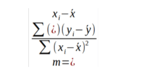
and the y-intercept c as:
c=y -mx (3)
where x and y are the average values of x and y variables, respectively.
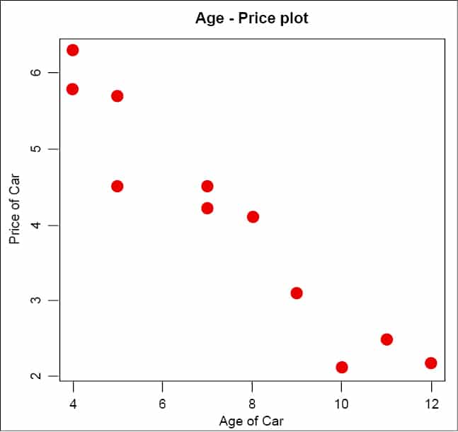
To illustrate the implementation of linear regression, let us consider an example of a simple relationship between a car’s age and its price. The relationship is depicted in a tabular form as shown below:
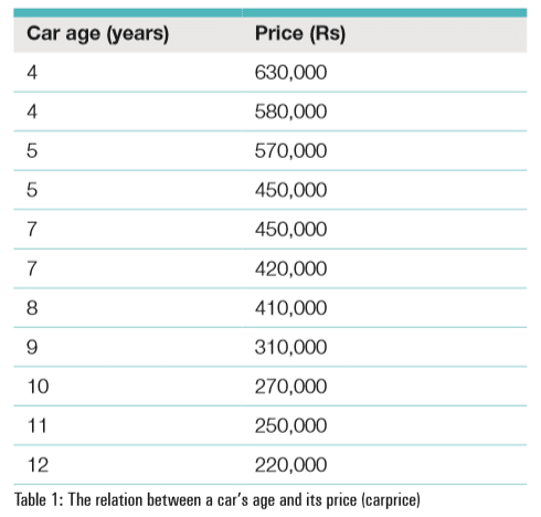
A table carprice has been created with a database dataanalysis, and used in an SQL query to determine regression analysis coefficients.
The task is to find the regression coefficients m and c using the formula given above. This can be done with other popular programming languages like R and Python, conveniently, through a language-specific RDBMS table import mechanism. With SQL, one can implement this directly within the database platform itself.
Implementation
SQL implementation of regression analysis is a straightforward exercise because the entire mathematical formulation can be implemented directly within the query. The query structure is a little cumbersome and requires attention. It need the sum of products, of different combinations. So, at the outset, let us try the slope alone. The slope variable m is the ratio of two sums of products of two different terms, and can be written in an SQL query as follows:
SELECT ROUND(
SUM(
(Age-(SELECT SUM(Age)/ COUNT(Age) AS avgAge FROM carprice))*
(Price-(SELECT SUM(Price)/ COUNT(Price) AS avgPrice FROM carprice))
)
/ SUM(
(Age-( SELECT SUM(Age)/ COUNT(Age) AS avgAge FROM carprice)) *
(Age-( SELECT SUM(Age)/ COUNT(Age) AS avgAge FROM carprice))
) ,2) AS m
FROM
carprice AS a;
If it is clear to you, you may now try the y-intercept c. It has three terms: y, x and m. Using the query expression of m, as stated in the previous query, we can write the following SQL statement for Equation 3.
SELECT round(
(SUM(Price)/ COUNT(Price)) - #y
(SUM #m
(
(Age-(SELECT SUM(Age)/ COUNT(Age) AS avgAge FROM carprice))*
(Price-(SELECT SUM(Price)/ COUNT(Price) AS avgPrice FROM carprice))
) /
SUM
(

(Age-(SELECT SUM(Age)/ COUNT(Age) AS avgAge FROM carprice)) *
(Age-(SELECT SUM(Age)/ COUNT(Age) AS avgAge FROM carprice))
)

)*

(SUM(Age)/ COUNT(Age)),2) as c #x
FROM
carprice AS test
The first query will return m as -0.50 and the second query will give c as 7.84. A negative slope value indicates lower values of the price with an increase in the age of the car. With the help of these two coefficients, one can estimate the selling price of a car if its age is given. For example, if the age of a car in the garage is three years, then the approximate price is:
SELECT -0.50*3+7.84 → 6.84 lakhs.
Both the coefficients in one query: A combined select query for the slope m and the y-intercept c can be written as follows:
SELECT
ROUND( #m
SUM(
(Age-(SELECT SUM(Age)/ COUNT(Age) AS avgAge FROM carprice))*
(Price-(SELECT SUM(Price)/ COUNT(Price) AS avgPrice FROM carprice))
)
/ SUM(
(Age-( SELECT SUM(Age)/ COUNT(Age) AS avgAge FROM carprice)) *

(Age-( SELECT SUM(Age)/ COUNT(Age) AS avgAge FROM carprice))
) ,2) AS m,

ROUND((SUM(Price)/ COUNT(Price)) - #c
(SUM(
(Age-(SELECT SUM(Age)/ COUNT(Age) AS avgAge FROM carprice))*
(Price-(SELECT SUM(Price)/ COUNT(Price) AS avgPrice FROM carprice))
)
/ SUM(
(Age-(SELECT SUM(Age)/ COUNT(Age) AS avgAge FROM carprice)) *
(Age-(SELECT SUM(Age)/ COUNT(Age) AS avgAge FROM carprice))
) )*
(SUM(Age)/ COUNT(Age)),2) AS c
FROM carprice
Like the earlier one, this query will also return -.50 and 7.84 for m and c, respectively.
The output is:
m c
-0.50 7.84
Estimate an unknown value
From the above three queries, we have seen how this complex query can be implemented in a step by step way. If the task is to implement Equation 1 directly in one go, then the equation can be written in SQL as follows:
set @testage=3
SELECT @testage*ROUND( #xm
SUM(
(Age-(SELECT SUM(Age)/ COUNT(Age) AS avgAge FROM carprice))*

(Price-(SELECT SUM(Price)/ COUNT(Price) AS avgPrice FROM carprice))
)

/ SUM(
(Age-( SELECT SUM(Age)/ COUNT(Age) AS avgAge FROM carprice)) *

(Age-( SELECT SUM(Age)/ COUNT(Age) AS avgAge FROM carprice))

) ,2) +
ROUND( #3
(SUM(Price)/ COUNT(Price)) -
(SUM(
(Age-(SELECT SUM(Age)/ COUNT(Age) AS avgAge FROM carprice))*

(Price-(SELECT SUM(Price)/ COUNT(Price) AS avgPrice FROM carprice))
) /

SUM(
(Age-(SELECT SUM(Age)/ COUNT(Age) AS avgAge FROM carprice)) *
(Age-(SELECT SUM(Age)/ COUNT(Age) AS avgAge FROM carprice))
) )*

(SUM(Age)/ COUNT(Age)),2) as y
FROM carprice
The age of a given car can be provided by defining an SQL variable @testage at the outset of the query as shown in the above example. After execution of this query, you will get 6.84 as the result of this query.
The output is:
y
6.84
For beginners, this query may be a bit cumbersome but a little care while writing such complex queries will give interesting results, and a sense of the power of SQL queries. This power of an elegant query can be further extended with R-SQL or Python-SQL.
Graphical analysis
The results of the above analysis can be studied with R or Python. Here, for better understanding, I have done the same exercise with R. The age and price attributes are assigned to x and y variables, respectively, and the slope variable m is calculated as defined in Equation 1.
#Age
>x=c(4,4,5,5,7,7,8,9,10,11,12)
#Price
>y=c(6.3,5.8,5.7,4.5,4.5,4.2,4.1,3.1,2.1,2.5,2.2)

#m = Equation(1)
#Numerator of equation 2

>num=sum((x-mean(x))*(y-mean(y)))
#Denominator of equation 2

>den=sum((x-mean(x))^2)
#m=Numerator/Denominator (Equation 1)
>m=num/den
#Equation(3)
>c = mean(y)-m*mean(x)
#Print the slop and interception values
>print(paste(“Slop (m)=”,round(m,2),”y-intercept (c)= “,c))

[1] “Slop (m)= -0.5 y-intercept (c)= 7.84
This finding may be verified using the R linear regression function lm() as given below:
#Regression using lm() function

>r=lm(y~x)

> summary(r)

Call:
lm(formula = y ~ x)

Residuals:
Min 1Q Median 3Q Max
-0.8241 -0.1669 0.1807 0.3295 0.4734

Coefficients:
Estimate Std. Error t value Pr(>|t|)
(Intercept) 7.8363 0.4118 19.027 1.41e-08 ***
x -0.5024 0.0520 -9.662 4.76e-06 ***
---

Signif. codes: 0 ‘***’ 0.001 ‘**’ 0.01 ‘*’ 0.05 ‘.’ 0.1 ‘ ’ 1

Residual standard error: 0.4614 on 9 degrees of freedom


Multiple R-squared: 0.9121, Adjusted R-squared: 0.9023
F-statistic: 93.35 on 1 and 9 DF, p-value: 4.76e-06
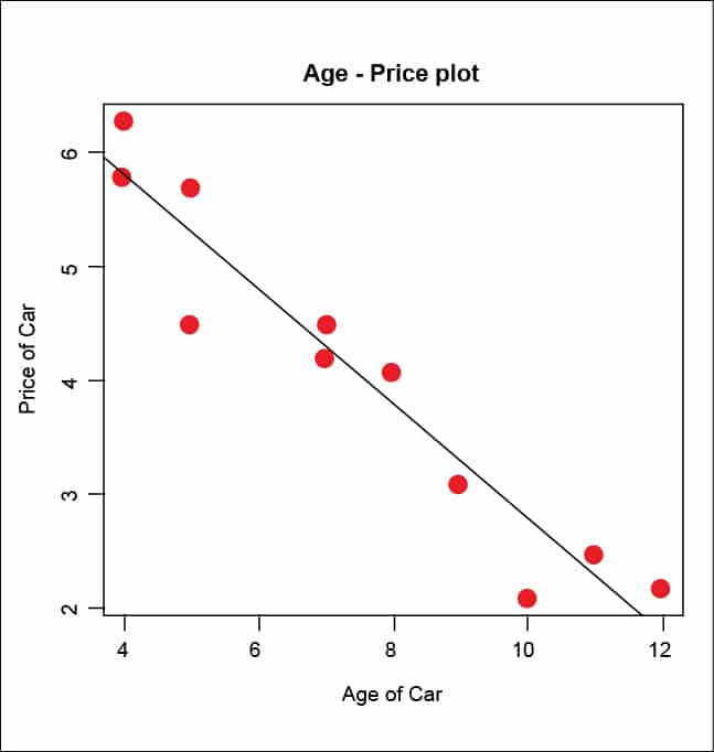
These values of linear regression of the car’s age and price can be further analysed using R plots and an overlaid linear regression slope line using the abline() function.
> plot(x,y,xlab=’Age of Car’,ylab=’Price of Car’,main=”Age - Price plot”,col=’red’,cex=2,pch=19)
> abline(r,col=”blue”,lw=2)
The scatter plot and regression line (Figure 2) clearly show a linear relationship between the age and price variables, and the slope indicates a decrease in the car’s price with the increase in its age.


