


Effective handling of data is very important for the success of any software application.
If a language provides an option to efficiently handle in-memory tabular data, it will make a developer’s life simple. This article introduces DataFrames.jl, an excellent package that you can use with Julia to handle in-memory tabular data, and explores its rich set of features.
Data is the lifeline of any software application. The success or failure of an application depends on the efficiency with which the data is represented and handled by it. During the earlier days, we had data structures such as arrays to handle a collection of homogenous data. When it comes to two-dimensional data, there are matrices that are built using two-dimensional arrays. Multi-dimensional data can be handled with multi-dimensional arrays.
Tabular data is one of the common types of data that we frequently encounter in real-time applications. Though we can handle tabular data with plain matrices, there are certain limitations in terms of the operations that we can do directly. To make the in-memory tabular data handling simpler, Julia has provided a very effective package called DataFrames.jl. This article explores the features of DataFrames.jl, and illustrates the preliminary steps involved in the efficient handling of tabular data using this software.
(If you are new to the Julia programming language, then you might consider reading this article, which introduces Julia, at https://www.opensourceforu.com/2016/10/julia-language/. Julia is a powerful language, and it is getting popular in various domains.)
Getting ready with DataFrames.jl
Any package in Julia is added using Pkg and add. Similarly, DataFrames.jl can also be added with the following commands:
using Pkg
Pkg.add(“DataFrames”)
The code shown in this article has been checked with Julia version 1.4.2.
To use DataFrames.jl, just place the following statement at the beginning of your code:
using DataFrames
What is a DataFrame?
A DataFrame is used to represent tabular data. It is represented as a series of vectors. These vectors represent columns. The easiest way to construct a DataFrame is to supply the column vectors. A sample is given below:
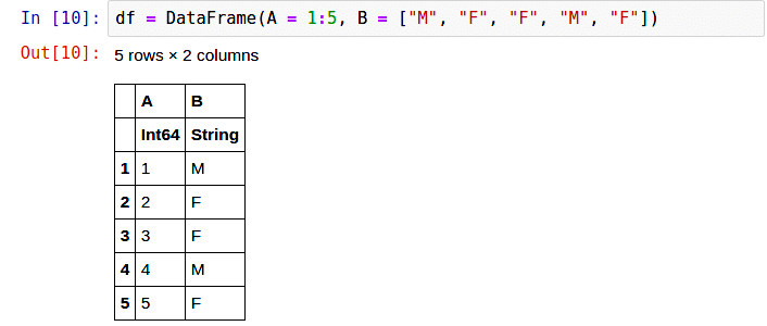
df = DataFrame(A = 1:5, B = [“M”, “F”, “F”, “M”, “F”])
Here we are building the DataFrame using two columns — A and B. Column A holds values from one to five, and column B has ‘M’ and ‘F’ as values. The output is shown in Figure 1.
Once the DataFrame is built, the individual columns can be accessed with the help of column names. For example:
df.A
5-element Array{Int64,1}:
1
2
3
4
5
DataFrames.jl supports both symbol representation and string representation for column names. The string representation of the column name is given within quotes, as shown below:
df.”A”
5-element Array{Int64,1}:
1
2
3
4
5
The individual column names can be fetched using the names() function:
2-element Array{String,1}:
“A”
“B”
If you want the same thing to be represented as a symbol, use the propertynames() function:
propertynames(df)

2-element Array{Symbol,1}:
:A
:B
Passing a single value
Julia allows the passing of a single value to a column, as shown in the following example:
df = DataFrame(“Magazine” => “OSFY”, “Theme” => [“Mobile”,”Cloud”,”Top10”, “Web”])
print(df)
The output is shown below:
4×2 DataFrame
│Row│ Magazine│ Theme  │
│   │ String  │ String │
├───┼────────┼─────────┤
│ 1 │ OSFY   │ Mobile  │
│ 2 │ OSFY   │ Cloud   │
│ 3 │ OSFY   │ Top10   │
│ 4 │ OSFY   │ Web     │
Column by column approach
In DataFrames, columns can be added individually:
df = DataFrame()
df.Month_Id = 1:12
df.Month_Name = [“Jan”, “Feb”, “Mar”, “Apr”, “May”, “Jun”, “Jul”, “Aug”, “Sep”, “Oct”, “Nov”, “Dec”]
print(df)
The output is shown below:
12×2 DataFrame
│ Row │ Month_Id │ Month_Name │
│     │ Int64    │ String     │
├─────┼──────────┼────────────┤
│ 1   │   1      │ Jan        │
│ 2   │   2      │ Feb        │
│ 3   │   3      │ Mar        │
│ 4   │   4      │ Apr        │
│ 5   │   5      │ May        │
│ 6   │   6      │ Jun        │
│ 7   │   7      │ Jul        │
│ 8   │   8      │ Aug        │
│ 9   │   9      │ Sep        │
│ 10  │   10     │ Oct        │
│ 11  │   11     │ Nov        │
│ 12  │   12     │ Dec        │
The size of the DataFrame may be fetched with the size() function:
size(df)
(12, 2)
Row by row approach
The DataFrame can be built in a row by row manner as well. The row can be added with the push() function, as shown below:
dframe = DataFrame(A = Int[], B = String[])
push!(dframe, (1, “January”))
push!(dframe, (1, “February”))
print(dframe)
The output is:
2×2 DataFrame
│ Row │ A     │ B       │
│     │ Int64 │ String  │
├─────┼───────┼─────────┤
│ 1   │ 1     │ January │
│ 2   │ 1     │ February│
Populating with random values
A DataFrame can be populated with random values by simply using the following code snippet:
df = DataFrame(rand(3,2))
print(df)
The output of the aforementioned code is:
3×2 DataFrame
│ Row│ x1       │ x2       │
│    │ Float64  │ Float64  │
├────┼──────────┼──────────┤
│ 1  │ 0.235304 │ 0.664924 │
│ 2  │ 0.0916205│ 0.131976 │
│ 3  │ 0.136018 │ 0.127914 │
Copying and comparison of DataFrames
A DataFrame object can be passed as an argument for building another DataFrame. Two DataFrames can be compared with is_equal(), as shown below:
df_one = DataFrame(a=1:5, b=’p’:’t’)
df_two = DataFrame(df_one)
print(df_two)
isequal(df_one,df_two)
Here, df_two is built as a copy of the df_one DataFrame. Then, these two DataFrames are compared, and the output (true) is shown.
The output of this code is shown below:
5×2 DataFrame
│ Row  │ a     │  b   │
│      │ Int64 │ Char │
├──────┼───────┼──────┤
│ 1    │ 1     │ ‘p’  │
│ 2    │ 2     │ ‘q’  │
│ 3    │ 3     │ ‘r’  │
│ 4    │ 4     │ ‘s’  │
│ 5    │ 5     │ ‘t’  │
true
Getting summary statistics
Getting the summary statistics of the data populated in a DataFrame is done with the describe() function. The describe() function provides the following statistics:
- Mean
- Minimum
- Median
- Maximum
- Number of unique values
- Number of missing values
- Data type
For example:
df = DataFrame(one = [1, 2], two = [5.0, missing], three = [“x”, “y”])
describe(df)
The output is shown in Figure 2.
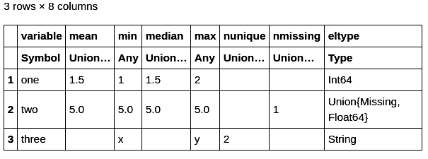
In this example, missing represents the missing value. You can supply specific column names to restrict the columns for which the summary statistics would be built, as shown below:
describe(df, cols=1:2)
Here, the summary statistics are built for the first two columns.
Selecting the first few rows
The first few rows of DataFrames can be selected using the first() function, as shown below:
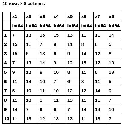
df = DataFrame(rand(5:15, 5000, 8))
first(df, 10)
Here we are building a DataFrame with 5000 rows and eight columns. Each cell is filled with a random value between five and 15. Then, the first ten rows are selected with the first(df,10) function. The output is shown in Figure 3.
Similarly, the last few rows can be fetched with the last() function:
last(df, 10)
If the first() and last() are supplied without the second argument, then the first and last rows are displayed. Here, only one row will be displayed.
Fetching specific columns
DataFrames.jl provides so many different options to fetch specific columns. Covering all of them would be out of the scope of this article. You are encouraged to refer to the official documentation for the complete list. Here, only sample methods are provided:
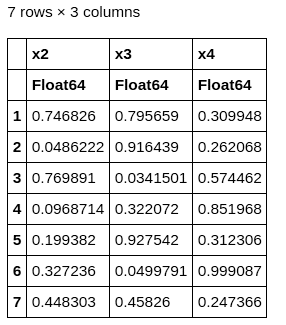
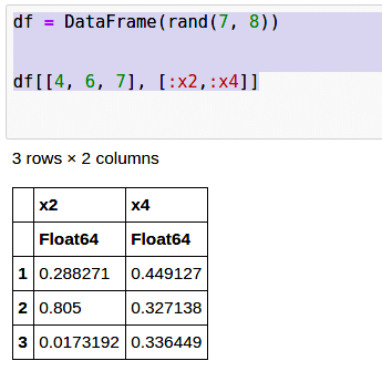
df = DataFrame(rand(7, 8))

df[:, Between(:x2, :x4)]
We have built a DataFrame with seven rows and eight columns with random values. By default, the column names are from x1 to x8. In this example, we have provided the command to fetch columns between x2 and x4. Here, the columns x2, x3 and x4 are fetched. The output is shown in Figure 4.
The column numbers can also be specified as given below:
df = DataFrame(rand(7, 8))
print(df[:, [3, 5]])
Here, columns 3 and 5 are displayed.
You can retrieve the specific rows and columns with the following syntax:
df = DataFrame(rand(7, 8))
df[[4, 6, 7], [:x2,:x4]]
Here, columns x2 and x4 are retrieved from rows 4, 6 and 7, as shown in Figure 5.
Grouping
groupby() is used to group values, as shown in the following example:
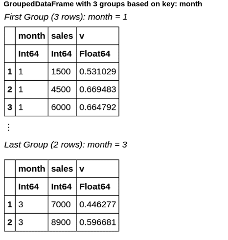
df = DataFrame(month=[1,2,1,2,3,1,3,2], sales=[1500, 3000, 4500, 8500, 7000, 6000, 8900, 7500], v=rand(8))
groupby(df, :month)
The output with the values grouped by the ‘month’ column is shown in Figure 6.
During Groupby, sorting can be done, and missing values can also be handled (Figure 7).
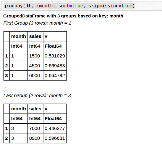
groupby(df, :month, sort=true, skipmissing=true)
As stated earlier, the objective of this article is to introduce the features of DataFrames.jl. For the complete enumeration of all the features, interested readers may refer to the official documentation. DataFrames.jl, with the lightning execution speed of Julia, is a great toolkit if you are handling data-intensive applications. Try exploring DataFrames.jl further with a free course (https://juliaacademy.com/p/introduction-to-dataframes-jl) from the Julia academy.


