


Julia is a high level, dynamic and general-purpose programming language. While it can be used for multiple purposes, it is most suited for complex numerical data analytics. This makes Julia an ideal language for implementing machine learning models. In this article, we will demonstrate how Julia can be used for machine learning.
First launched in 2012, Julia has become one of the top emerging open source programming languages to learn in 2021 and beyond. This is because Julia, by design, is a language that is ideal for complex analysis of numerical data. With the rise of data science (DS) and cloud computing, and the abundance of Big Data, Julia is becoming more and more relevant and necessary for the ML/DS community. In this article, our focus will be to demonstrate how you can get started with machine learning (ML) using Julia. Julia is astonishingly similar to Python when it comes to the syntax of the code. This makes the language quick to grasp and easy to implement for most developers.
Instead of taking you through the rather self-explanatory installation process or the basics of the language, I am going to jump-start this article by taking you directly to the good stuff. We will learn how to use Julia for machine learning by implementing a linear regression model to predict the house prices in Boston, Massachusetts, USA.
Why use Julia for machine learning?
Before jumping into the implementation part, let me list out a few reasons why you should consider using Julia for machine learning. After all, in a world where there is Python and R, why would you want to add another language to perform the same tasks? Here’s why:
- It is open source and free to use under the MIT licence.
- Julia is faster than Python and R. Yes, you read that right. Julia is by design faster at executing complex mathematical formulae as this was the original purpose behind creating the language.
- Julia supports concurrent parallel and distributed computing.
- Julia has the ability to directly call C or Fortran code without the requirement of additional glue code.
- Julia uses the ‘Just Ahead of Time’ (JAOT) compiler, which compiles the code to machine code by default before execution.
- Julia has some of the most efficient libraries for floating-point calculations and linear algebra (i.e., calculations involving matrices), which are essential for machine learning.
- Julia is supported by popular IDEs such as Visual Studio Code and execution environments such as Jupyter Notebook.
- It is super easy to install and get started.
- Julia has a vibrant online community that is active and increasing by the day.
Pre-requisites
Now that we have a pretty good grasp on what Julia is and what makes it ideal for machine learning, it’s time to get our hands dirty. In this section of the article, we are going to implement a simple linear regression model to help us predict the prices of houses in Boston, Massachusetts, USA.
There are a few pre-requisites that need to be taken care of before getting started with the implementation:
- Visit https://julialang.org/ and install the language in your OS. The procedure is pretty straightforward and Julia is available on all major platforms.
- Visit https://jupyter.org/ and install Jupyter Notebook in your OS. Again, the procedure is pretty easy to follow, so we do not need to go into too many details.
- You will also need the standard Boston house prices data set used to demonstrate linear regression. Visit https://www.kaggle.com/ to download.
- Now that we have taken care of the necessary pre-requisites for this demonstration, let’s get to the code.
Implementation
Developers familiar with Python are going to find many similarities in the syntax, structure and method of implementation in Julia. We will use a Jupyter Notebook for the compiling and execution of our code. So open up a fresh Jupyter Notebook in the desired folder and make sure to save your data set in the same location.
1. To start with, we are going to require certain libraries that we will make use of in this example. We will deal with data from a csv file. This will require us to use DataFrames. Additionally, we will perform some statistical calculations. Last but not the least, we will require a generalised linear model (GLM) for the implementation.
using DataFrames, CSV
using Plots
using GLM
using Statistics
using StatsPlots
2. Using the CSV and DataFrame libraries that we imported, we load the data from the data set.
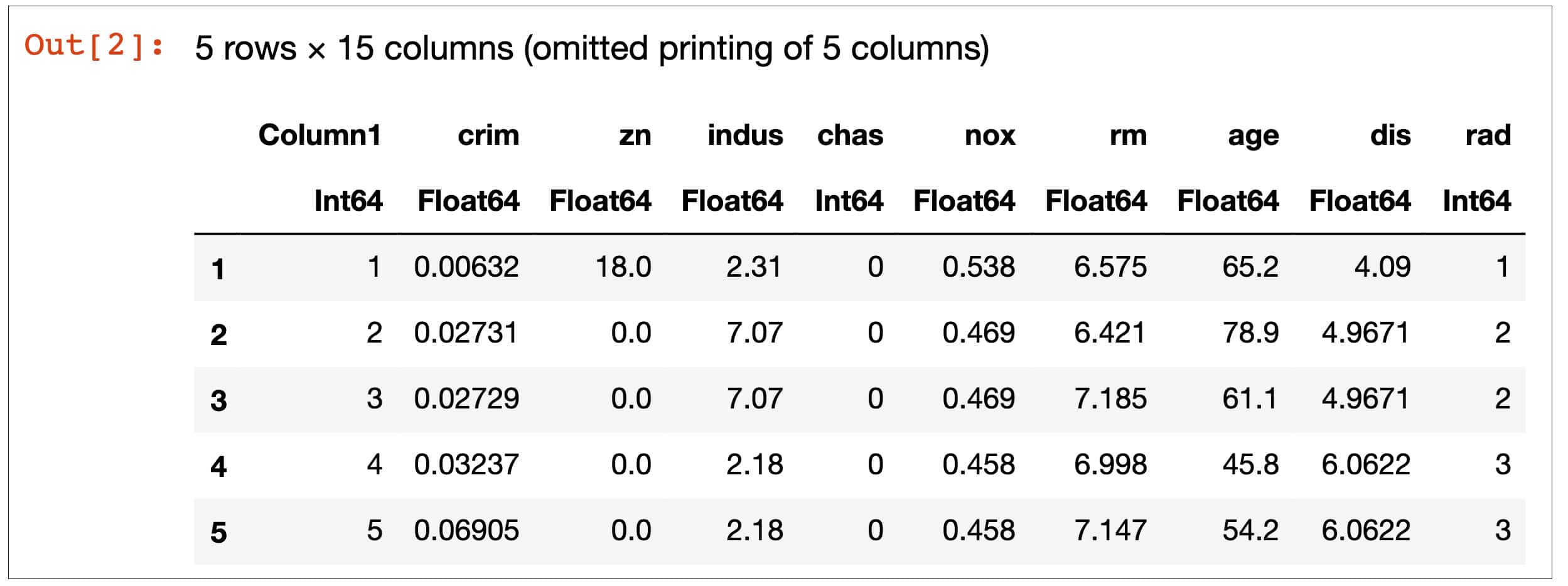
# Read the file using CSV.File and convert it to DataFrame
df = DataFrame(CSV.File(“Boston.csv”))
first(df,5) #displaying the first 5 rows to get an overview of the dataset
Figure 1 shows the first five rows of data in the form of a DataFrame. This helps us to understand the data has loaded properly.
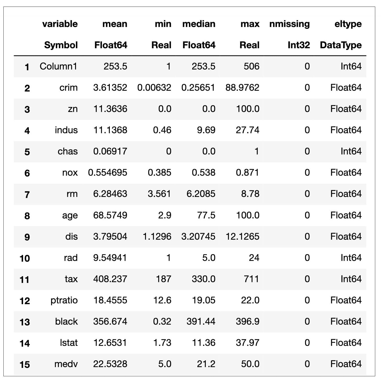
3. We can now explore this data set to find out its size, i.e., the number of rows and columns. We can also use the describe method to draw up some statistical data.
# Read the file using CSV.File and convert it to DataFrame
df = DataFrame(CSV.File(“Boston.csv”))
first(df,5) #displaying the first 5 rows to get an overview of the dataset
Figure 2 shows the statistical description of the data, i.e., mean, median, min, max, etc.
4. An important step before implementing the model is to divide the data set into features and target variable. We will take the target variable (house prices) on the Y list and the features on the X.
y = df[:, :medv]; #Y-values
X = select!(df, Not(:medv)); #features
5. In order to both train and test the model, we will need to divide the data set into training data and testing data. We will use 80 per cent of the data for training and the rest 20 per cent for testing.
design_matrix = convert(Matrix, X)
train_size = 0.80 #sepecifying the split ratio
num_samples = size(design_matrix)[1] #total number of samples in dataset

train_index = trunc(Int, train_size * num_samples) #truncating 80% of samples for training

# Split using the desired train size
X_train = design_matrix[1:train_index, :]
X_test = design_matrix[train_index+1:end, :]

y_train = y[1:train_index]
y_test = y[train_index+1:end]

print(“Dataset split into train and test”)
6. As a necessary pre-processing step, we will perform scaling and transformation on the training and testing data.
# defining function to scale features
function scale_features(X)

μ = mean(X, dims=1)
σ = std(X, dims=1)

X_norm = (X .- μ) ./ σ
return (X_norm, μ, σ)

end

#defining function to transform features.
function transform_features(X, μ, σ)
X_norm = (X .- μ) ./ σ
return X_norm
end

# Scale training features
X_train_scaled, μ, σ = scale_features(X_train)

# Transform the testing features
X_test_scaled = transform_features(X_test, μ, σ)

print(“Training and testing data are now transformed”)
7. We will also need to define a cost function for determining the mean squared error.
# compute cost function helps us to compute the mean squared error
function compute_cost(X, y, theta)
m = size(X)[1] # number of samples

preds = X * theta #calculate predictions using theta
loss = preds - y #calculate error

# Half mean squared loss
cost = (1/(2m)) * (loss’ * loss)
return cost

end
8. The cost function requires the theta value for making the predictions from which the error can be calculated. In order to update the theta value, we require the gradient descent function.
# Gradient Descent function to update the theta values
function gradient_descent(X, y, alpha, fit_intercept=true, n_iter=2000)

m = length(y) # number of training examples

if fit_intercept
# Add a bias
b = ones(m, 1)
X = hcat(b, X)
else
X
end

# Initializing theta
theta = zeros(size(X)[2])

# Initialise the cost vector
cost = zeros(n_iter)

#looping over the number of iterations
for iter in range(1, stop=n_iter)
pred = X * theta #predictions

# Calculate the cost for each iter
cost[iter] = compute_cost(X, y, theta)

# Update the theta θ at each iter
theta = theta - ((alpha/m) * X’) * (pred - y);
end
return (theta, cost)
end
9. Finally, we are ready to train the model with our scaled and transformed data set.
theta, cost = gradient_descent(X_train_scaled, y_train, 0.05, true, 1000)

# plot the cost during training
plot(cost,
label=”Cost per iter”,
ylabel=”Cost”,
xlabel=”Number of Iteration”,
title=”Cost Per Iteration”)
10. We will now make predictions on both the training and the testing data using our model.
# function used for prediction on given dataset using trained theta values
function predict(X, theta, fit_intercept=true)
m = size(X)[1]

if fit_intercept
b = ones(m)
X = hcat(b, X)
else
X
end

predictions = X * theta

return predictions
end

# Make predictions for both training and testing datasets
pred_train = predict(X_train_scaled, theta)
pred_test = predict(X_test_scaled, theta)

print(“Predictions made on the training and testing set”)
11. We have now reached the final step where we will verify the accuracy of our model by measuring the r-squared value of our predictions for the testing data.
#The function below returns the R squared value based on the predictions (y_pred) and the ground truth values (y_true)passed to it.

function r_squared_score(y_pred, y_true)

# Compute sum of explained variance (SST) and sum of squares of residuals
sst = sum(((y_true .- mean(y_true)) .^ 2))
ssr = sum(((y_pred .- y_true) .^ 2))

r_square = 1 - (ssr / sst)

return r_square
end

# Get the r-squared score for training and test datasets
train_r_square = r_squared_score(pred_train, y_train)

println(“Training R square score for test sets: “, train_r_square)
Figure 3 shows us the r-square score for the model which can be rounded to about 0.73. In this demonstration, we trained the linear regression model from scratch. Of course, just like Python, you always have the option to use the model directly from the stats package in Julia. That way, you can execute this entire process in four lines of code.

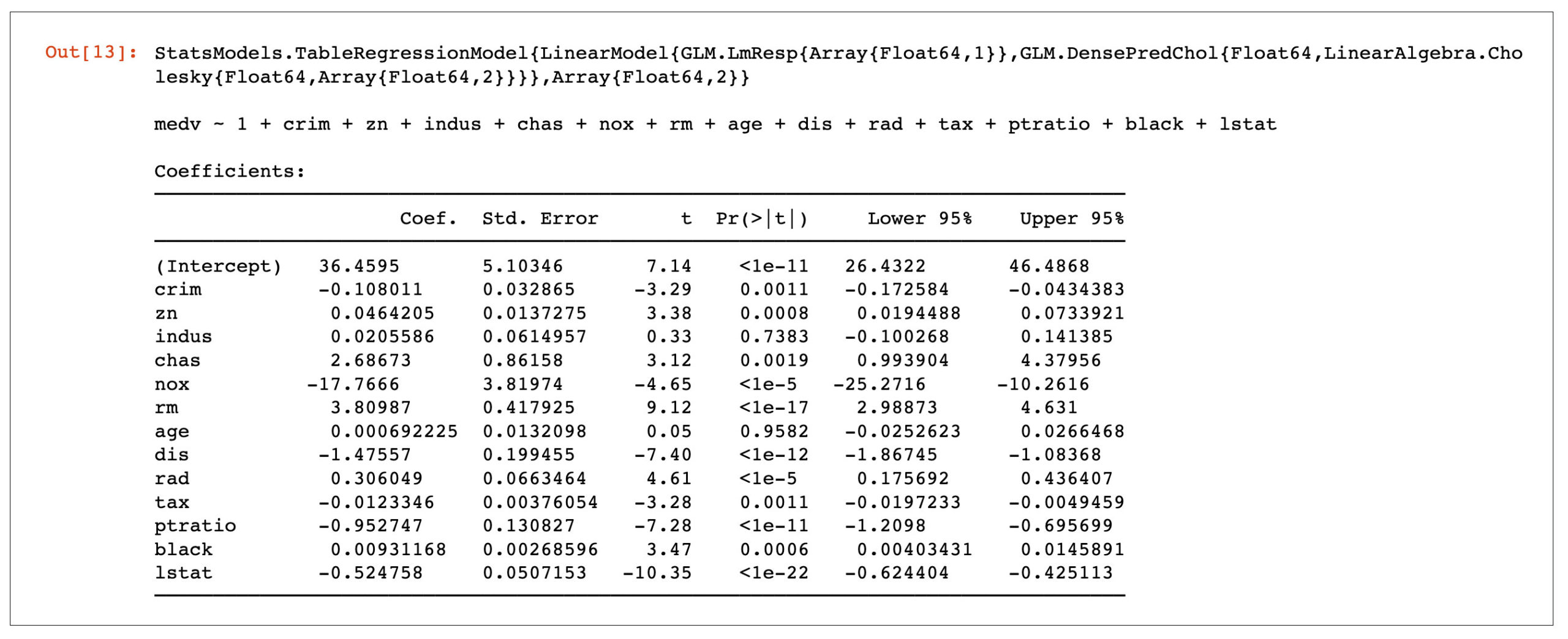
df = DataFrame(CSV.File(“Boston.csv”))
fm = @formula(medv ~ crim +zn+indus+chas+nox+rm+age+dis+rad+tax+ptratio+black+lstat)
linearRegressor = lm(fm, df)
Figure 4 shows us the coefficients that are derived using the linear regression model from the stats package. Let us now calculate the r-square for this model:
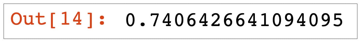
# R Square value of the model
r2(linearRegressor)
From Figure 5, it becomes abundantly clear that it doesn’t make much of a difference whether you train data from scratch or use the more convenient approach of using a regression model from the stats package. The difference between both the r-squared scores, i.e., 0.73 and 0.74, is negligible.
In this article, we implemented a linear regression model using the Julia programming language to predict prices in the housing market of Boston, Massachusetts, USA. This article has been written to give you a taste of the Julia programming language. The example used is but a simple demonstration of the power of Julia. If you are coming from a Python background, then you are most certainly going to find many similarities between the two languages in terms of syntax, structure and approach. This is good news as the learning curve is less.
It is my opinion that Julia is a must have on your resume, whether you are a practising or a prospective data scientist.


