


In this third article in the ‘R, Statistics and Machine Learning’ series, we shall explore the various data structures such as vectors, arrays, matrices, lists, factors and data frames that are provided in R to represent data.
We will be using R version 4.1.0 installed on Parabola GNU/Linux-libre (x86-64) for the code snippets. You can just check the version by typing:
$ R --version
Vector
A vector is a collection that contains a single type of value. It can be numerical, a character, floating point, complex number or have logical values. For example:
> c(1, 2, 3, 4)
[1] 1 2 3 4
Operations can be performed on vectors. An addition operation is shown below:
> c(1, 2, 3, 4) + c(1, 1, 1, 1)
[1] 2 3 4 5
If the size of the vectors is not equal in the operation, the smaller sequence is repeated to fill-in, as illustrated below:
> c(1, 2, 3, 4) + c(1, 1)
[1] 2 3 4 5

> c(1, 2, 3, 4) + c(1)
[1] 2 3 4 5
You can apply a filter selection, and only those vector members that satisfy the condition are returned. In the following example, only the indices that are divisible by two are listed:
> n <- c(1, 2, 3, 4)
> n[n %% 2 == 0]
[1] 2 4
The use of negative indices wraps around the vector boundary limits, as shown below:
> n[-1:-2]
[1] 3 4
An example of character (string) vector in R is as follows:
> c(“One”, “Two”, “Three”, “Four”)
[1] “One” “Two” “Three” “Four”
You can retrieve members by specifying an index or an index range for the vector. A couple of examples are given below:
> v <- c(“One”, “Two”, “Three”, “Four”)

> v[1]
[1] “One”

> v[1:3]
[1] “One” “Two” “Three”
In the above example, the vector represents a character vector.
> typeof(v)
[1] “character”
You can also use logical values in a vector. For example:
> b <- c(TRUE, FALSE)

> b
[1] TRUE FALSE

> typeof(b)
[1] “logical”
The R ifelse is a conditional element selection function. An example is given below to illustrate its use:
> p <- c(“0”, “0”, “1”, “1”)

> q <- c(“0”, “1”, “0”, “1”)

> ifelse(c(FALSE, FALSE, TRUE, TRUE), p, q)
[1] “0” “1” “1” “1”
Array
An array is a multi-dimensional vector where you can explicitly define the dimensions. For example:
> a <- array(c(1, 2, 3, 4, 5, 6, 7, 8, 9), dim=c(3, 3))
> a
[,1] [,2] [,3]
[1,] 1 4 7
[2,] 2 5 8
[3,] 3 6 9
You can retrieve a member by specifying the indices within a square parenthesis:
> a[2,3]
[1] 8
You can also mention a range of indices. For example:
> a[1:2, 1:2]
[,1] [,2]
[1,] 1 4
[2,] 2 5
The following construct returns all the values for the first row:
> a[1,]
[1] 1 4 7
You can specify the column number to return all its values as well:
> a[,2]
[1] 4 5 6
The output can be delimited by specifying an index range, as shown below:
> a[2:1, ]
[,1] [,2] [,3]
[1,] 2 5 8
[2,] 1 4 7
The following is an example of a 2x2x2 multi-dimensional array construction:
> m <- array(c(1, 2, 3, 4, 5, 6, 7, 8), dim=c(2, 2, 2))
> m
, , 1

[,1] [,2]
[1,] 1 3
[2,] 2 4

, , 2

[,1] [,2]
[1,] 5 7
[2,] 6 8
You can again specify the indices for the various dimensions to retrieve the values from the defined array:
> m[1, 1, 1]
[1] 1
For the given example, the values in ‘a’ are represented as a double.
> typeof(a)
[1] “double”
The class of ‘a’ is a ‘matrix’ ‘array’.
> class(a)
[1] “matrix” “array”
Matrix
A matrix is a vector in two dimensions. You can use the matrix() function to create a new matrix, as shown below:
> m <- matrix(data=c(1, 2, 3, 4, 5, 6, 7, 8, 9), nrow=3, ncol=3)
> m
[,1] [,2] [,3]
[1,] 1 4 7
[2,] 2 5 8
[3,] 3 6 9
The ‘m’ matrix has a ‘double’ value as its type.
> typeof(m)
[1] “double”
You can of course retrieve the individual members in the matrix by specifying the indices.
> m[1]
[1] 1
You can retrieve the first row of the matrix similar to an array, as shown below:
> m[1,]
[1] 1 4 7
A range of indices can be supplied to the matrix to return the relevant elements:
> m[1:2, ]
[,1] [,2] [,3]
[1,] 1 4 7
[2,] 2 5 8
You can also specify all the dimensions to get a specific value present in a matrix cell:
> m[1,2]
[1] 4
The assignment operator can be used to update a specific value in the matrix, as shown below:
> m[1,2] <- 100
> m
[,1] [,2] [,3]
[1,] 1 100 7
[2,] 2 5 8
[3,] 3 6 9
You can also specify the dimension names when creating a matrix, as illustrated below:
> m <- matrix(data=c(1, 2, 3, 4, 5, 6, 7, 8, 9), nrow=3, ncol=3, dimnames=list(c(“r1”, “r2”, “r3”), c(“c1”, “c2”, “c3”)))

> m
c1 c2 c3
r1 1 4 7
r2 2 5 8
r3 3 6 9
The specific row names of the matrix can be displayed, as shown below:
> row.names(m)
[1] “r1” “r2” “r3”
The various attributes of the matrix can be obtained using the attributes() function:
> attributes(m)
$dim
[1] 3 3

$dimnames
$dimnames[[1]]
[1] “r1” “r2” “r3”

$dimnames[[2]]
[1] “c1” “c2” “c3”
List
Lists in R are different from vectors as they can contain different data types. For example, in the following example we have a number and two strings:
> l <- list(“R”, 28, “GPLv2”)
> l
[[1]]
[1] “R”

[[2]]
[1] 28

[[3]]
[1] “GPLv2”

> l[1]
[[1]]
[1] “R”
You can specify attribute names to the values when creating a list, as indicated below:
> l <- list(name=”R”, age=28, license=”GPLv2”)
> l
$name
[1] “R”

$age
[1] 28

$license
[1] “GPLv2”
The individual values from the list can be obtained with their respective attribute names, as follows:
> l$name
[1] “R”

> l$age
[1] 28

> l$license
[1] “GPLv2”
You can also concatenate lists together, as shown below:
> n <- list(list(name=”Clojure”, age=14, license=”Eclipse Public License”), l)
> n
[[1]]
[[1]]$name
[1] “Clojure”

[[1]]$age
[1] 14

[[1]]$license
[1] “Eclipse Public License”

[[2]]
[[2]]$name
[1] “R”

[[2]]$age
[1] 28

[[2]]$license
[1] “GPLv2”
The typeof() function returns the list type as a “list”:
> typeof(l)
[1] “list”

> typeof(n)
[1] “list”
You can retrieve the individual list entries using the indices, as illustrated below:
> n[1]
[[1]]
[[1]]$name
[1] “Clojure”

[[1]]$age
[1] 14

[[1]]$license
[1] “Eclipse Public License”
The second entry in the list ‘n’ with index ‘2’ is given below:
> n[2]
[[1]]
[[1]]$name
[1] “R”

[[1]]$age
[1] 28

[[1]]$license
[1] “GPLv2”
In a list of lists, you can obtain the value by enclosing the name attribute within double square parentheses.
For example:
> l[[“name”]]
[1] “R”
A list can be converted to a vector using the unlist() function. The assignment operator can be used to update a value in a list. An example is given below:
> l <- list(“R”, 28, “GPLv2”)
> l[3] <- “GNU GPLv2”
> l
[[1]]
[1] “R”

[[2]]
[1] 28

[[3]]
[1] “GNU GPLv2”
Factors
A factor is an ordered collection of entities that are used to represent categories. Although you can use vectors for the same, these can be inefficient for large data. You can use the factor() function to create a factor. For example:
> gender <- factor(c(“male”, “female”, “male”, “female”, “male”))
> gender
[1] male female male female male
Levels: female male
The different values that a factor can take are known as levels. The factors are actually stored internally as integer vectors. This can be seen using the str() function:
> str(gender)
Factor w/ 2 levels “female”,”male”: 2 1 2 1 2
If you try to apply the min() function for the above categorical values, R will throw an error. You need to use the ordered flag to indicate that there is a logical ordering to the categories. For example:
> room <-factor(c(“standard”, “premium”, “luxury”), ordered = TRUE)
> room
[1] standard premium luxury
Levels: luxury < premium < standard
The various levels for the room example are shown below:
> levels(room)
[1] “luxury” “premium” “standard”

> nlevels(room)
[1] 3
You will now be able to apply the min() function to the room factor to return valid levels, as illustrated below:
> min(room)
[1] luxury
Levels: luxury < premium < standard
Data frames
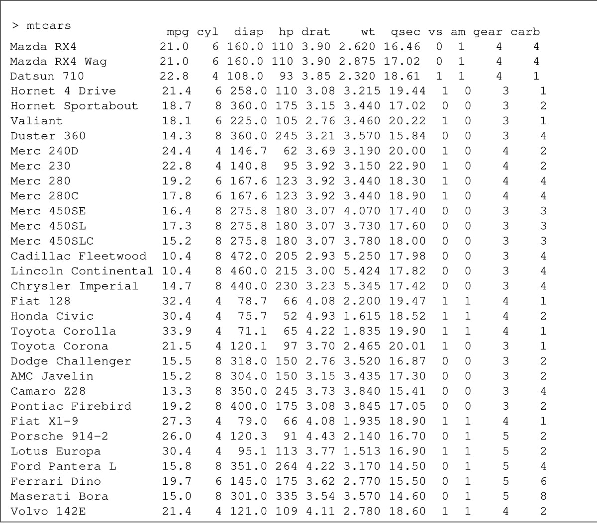
A data frame contains a number of named vectors that have the same length. These frames are internally built on R lists. The mtcars data set in R provides Motor Trend Car Road Test information from the 1974 Motor Trend US magazine (Figure 1). It has information on 11 numeric values such as miles/(US) gallon (mpg), number of cylinders (cyl), displacement (cu.in) (disp), horsepower (hp), rear axle ratio (drat), weight (1000 lbs) (wt), 1/4 mile time (qsec), engine (0 = V-shaped, 1 = straight) (vs), transmission (0 = automatic, 1 = manual) (am), number of gears (gear) and carburetor (carb).
We can create a data frame with a sample set from the mtcars data set as follows:
> name <- c(“Mazda RX4”, “Mazda RX4 Wag”, “Datsun 710”, “Hornet 4 Drive”, “Hornet Sportabout”, “Valiant”)
> name
[1] “Mazda RX4” “Mazda RX4 Wag” “Datsun 710”
[4] “Hornet 4 Drive” “Hornet Sportabout” “Valiant”

> mpg <- c(21.0, 21.0, 22.8, 21.4, 18.7, 18.1)
> mpg
[1] 21.0 21.0 22.8 21.4 18.7 18.1

> cyl <- c(6, 6, 4, 6, 8, 6)
> cyl
[1] 6 6 4 6 8 6

> disp <- c(160, 160, 108, 258, 360, 225)
> disp
[1] 160 160 108 258 360 225

> hp <- c(110, 110, 93, 110, 175, 105)
> hp
[1] 110 110 93 110 175 105

> wt <- c(2.620, 2.875, 2.320, 3.215, 3.440, 3.460)
> wt
[1] 2.620 2.875 2.320 3.215 3.440 3.460

> gear <- c(4, 4, 4, 3, 3, 3)
> gear
[1] 4 4 4 3 3 3

> cars <- data.frame(name, mpg, cyl, disp, hp, wt, gear)
> cars
name mpg cyl disp hp wt gear
1 Mazda RX4 21.0 6 160 110 2.620 4
2 Mazda RX4 Wag 21.0 6 160 110 2.875 4
3 Datsun 710 22.8 4 108 93 2.320 4
4 Hornet 4 Drive 21.4 6 258 110 3.215 3
5 Hornet Sportabout 18.7 8 360 175 3.440 3
6 Valiant 18.1 6 225 105 3.460 3
>
The type of ‘cars’ is a list.
> typeof(cars)
[1] “list”
The structure of the data frame can be seen using the str() function, as illustrated below:
> str(cars)
‘data.frame’: 6 obs. of 7 variables:
$ name: chr “Mazda RX4” “Mazda RX4 Wag” “Datsun 710” “Hornet 4 Drive” ...
$ mpg : num 21 21 22.8 21.4 18.7 18.1
$ cyl : num 6 6 4 6 8 6
$ disp: num 160 160 108 258 360 225
$ hp : num 110 110 93 110 175 105
$ wt : num 2.62 2.88 2.32 3.21 3.44 ...
$ gear: num 4 4 4 3 3 3
You can retrieve the individual values using indices for the data frame. You can also specify a range for the indices, as shown below:
> cars[1:2, 2]
[1] 21 21
The column values can be obtained by mentioning the column name in the data frame. For example:
> cars[, “wt”]
[1] 2.620 2.875 2.320 3.215 3.440 3.460

> cars$wt
[1] 2.620 2.875 2.320 3.215 3.440 3.460
You can also retrieve a section of the data that satisfies a condition using the subset() function, as illustrated below:
> subset(cars, subset = hp > 100)
name mpg cyl disp hp wt gear
1 Mazda RX4 21.0 6 160 110 2.620 4
2 Mazda RX4 Wag 21.0 6 160 110 2.875 4
4 Hornet 4 Drive 21.4 6 258 110 3.215 3
5 Hornet Sportabout 18.7 8 360 175 3.440 3
6 Valiant 18.1 6 225 105 3.460 3
The cars can be sorted based on the displacement data in ascending order using the order() function, as shown below:
> order(cars$disp)
[1] 3 1 2 6 4 5
You are encouraged to try the above data structures and their supported functions on your data to understand their use and functionality. In the next part, we shall learn how to import data from various sources into R.


