Exploratory data analysis (EDA) reveals the internal pattern of data. It is often used to validate hypotheses, verify certain theories and explore data sets in order to find the distribution pattern of the sample collected. Summary statistics and visualisation of data are two frequently used data analysis parameters, which often help businesses to decide future courses of action.
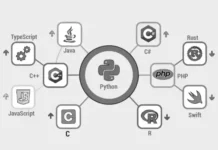
In general, data is available in different forms and most of it is unstructured. For efficient and stable data processing, a primary requirement is to organise data into a well-defined form. Relational database management systems (RDBMSs) play this role and currently, MySQL is one of the most used among them. It provides a well-defined structured storage platform for data and forms the basis of exploratory data analysis or EDA. It also supports the conversion of different forms of data into its own form and vice versa. Data collected from other platforms may need to be refined and cleaned, and MySQL’s pattern recognition, filtering and conversion tools are helpful in this respect. Moreover, its strong interface with other programming language platforms like R, Python and PHP makes it a robust and most efficient EDA platform.
EDA with MySQL takes place over the following four steps:
- The collection of data from different platforms
- The cleaning and validation of data
- Analysis of data
- The export of data to other platforms for further analysis
Importing files
Since records of an organisation are always stored in different forms — starting from handwritten ledgers to WhatsApp communications, it’s a Herculean task to convert data in these disparate formats into a structured form for an integrated higher-level analysis. MySQL supports conversion of data from Microsoft Excel, CSV, XML and pure text data to its own structured format. It also supports exporting of its own data to these forms. Here are some data importing functions and their syntax in the form of examples.
An example for CSV and Excel files:
LOAD DATA LOCAL INFILE ‘/path/to/your/csv/file/mydata.csv’

INTO TABLE database.table

FIELDS TERMINATED BY ‘,’ ENCLOSED BY ‘”’ LINES TERMINATED BY ‘\n’;
An example for XML files:
LOAD DATA LOCAL INFILE ‘/path/to/your/csv/file/mydata.xml’

INTO TABLE database.table

ROWS IDENTIFIED BY ‘<tag>’
It’s obvious that for a database, a table has to be created before loading the data into it. Moreover, the table’s structure should be compatible with the data that is to be loaded. For importing Excel data, the best way is to convert the Excel worksheet into a CSV file. This process filters out all the unprintable characters and meta data from the sample, making it ready for the SQL format.
Processing and filtering of data
This step is essential for further high-level analysis of data. Since SQL queries work on data of a particular format and the supporting data structures, filtering of data not only helps to eliminate unwanted errors but also to understand the data better. Among different data types, floating point numbers should be in proper format, and time-date data should be according to MySQL’s YYYY-MM-DD format. Care is required to handle the null values also. There are a few SQL functions for identifying and subsequently cleaning the imported data. These functions are LIKE(), TRIM(), REPLACE(), LEFT(), RIGHT(), CONCAT(), UPPER(), LOWER(), and FORMAT(). The most important SQL tools to handle data filtering dynamically are COALESCE and CASE-END statements. These have two forms — Search CASE, which is used in SQL query statements, and Simple CASE, which is used in stored programming.
In the cleaning process, the following needs to be taken care of:
- Formats of data
- Formats of decimal data
- Misspelt and mistyped data
- Null field values
Formats of imported data should match the SQL table format, and care should be taken while preparing data and the SQL tables. A NULL value field option can be incorporated into the SQL table structure itself. Spelling and other data arrangements can be handled with SQL functions like TRIM(), LEFT(), RIGHT(), UPPER(), CONCAT(), etc.
Higher-level dynamic filtering can be implemented using COALESCE and CASE-END statements. For instance, to filter a GENDER field with values like ‘M’, ‘Male’, ‘F’, ‘Female’, 0 and 1, COALESCE-CASE statements can be used to normalise the data as follows:
SELECT adm_no,stu_name,COALESCE(
CASE WHEN sex=”M” THEN “Male” ELSE NULL END,
CASE WHEN sex=”Male” THEN “Male” ELSE NULL END,
CASE WHEN sex=”F” THEN “Female” ELSE NULL END,
CASE WHEN sex=”Female” THEN “Female” ELSE NULL END,
cASE WHEN sex=”0” THEN “Male” ELSE NULL END,
CASE WHEN sex=”1” THEN “Female” ELSE NULL END
)
from STUDENTS
WHERE id >= 33 and id <= 42;

Adm_no Name Gender
613121 HARI KANT GAUTAM Male
613168 SANGRAM RAY Male
613177 S.K. HAFIZUL ISLAM Male
613183 KAILASH KUMAR Female
613216 BRIJENDRA KUMAR Female
613238 DAMODAR REDDY EDLA Female
613240 M.RAJASEKHAR REDDY Tran
613122 SUNIL KUMAR SHARMA Male
613146 RAJIV CHOUDHARY Male
Another useful filtering tool is the CONVERT() function. It is used to convert one data type to another. For example, to convert a string date field value to the MySQL date format YYYY-MM-DD, CONVERT can be used as follows:
SELECT CONVERT(‘2014-02-28 08:14:57’, DATETIME);
Result: ‘2014-02-28 08:14:57’
Data processing and visualisation
After collecting, arranging and cleaning data, we are now ready to process it. The goal of processing the data is to extract meaningful information from it. Proper analysis provides insights into the business process and helps the management to take proper decisions. Here I have considered the Northwind database for analysis. As I have already discussed data analysis using SQL, I will extend the data analysis paradigm from MySQL to R, so that readers can get an idea of the full potential of a data analysis platform.
Data can be exported from MySQL to R, as follows:
library(RMySQL)
mydb = dbConnect(MySQL(), user=’root’, password=’root’, dbname=’northwind’)

rs = dbSendQuery(mydb, “select * from invoices”)

data = fetch(rs,-1)
Exporting data to R
The R library, RMySQL, supports a full range of simple and complex SQL queries. For example, if you need to analyse data about the orders received by your organisation, with all the details from other tables, you can write an SQL query as follows:
sqlstr=”
SELECT
o.OrderID
, p.ProductName
, p.ProductID
, od.UnitPrice
, od.Quantity
, od.UnitPrice * od.Quantity AS subtotal
, c.CustomerID
, s.SupplierID
FROM orderdetails AS od

LEFT JOIN Orders AS o ON od.OrderID = o.OrderID

LEFT JOIN Products AS p ON p.ProductID = od.ProductID

LEFT JOIN Customers AS c on c.CustomerID = o.CustomerID
LEFT JOIN Suppliers AS s ON s.SupplierID = p.SupplierID; “
And we can execute the query with R as:
rs = dbSendQuery(mydb, sqlstr)
data = fetch(rs,-1)

> head(data)
Visualisation
Let us look at an example of data analysis and visualisation. To get a frequency distribution of ordered products, a merger of the order details and products table can be done as follows:
>>>sqlstr=”
select a.ProductId,b.ProductName,(a.ProductId) As Frequency
from orderdetails as a
inner join products as b on b.ProductID=a.ProductID
group by ProductID;”
rs = dbSendQuery(mydb, sqlstr)
data = fetch(rs,-1)
Since the query returns three fields, i.e., ProductID, ProductName and Frequency, a histogram of the frequency distribution of products can be written in R as shown below:
>>>names(data)
[1] “ProductId” “ProductName” “Frequency”
hist(data$Frequency,col = “green”,border = “red”, xlim = c(1,77), main=’Histogram of Products’,xlab=”Products”, ylab=”Frequency”)
Here are some simple tips to perform a few common data analysis tasks.
- To get the top ten results, one can sort the record sets with DESC and LIMIT the report for the top ten records.
- To get the statistical analysis of different fields of sales and marketing data, one can use statistical functions like AVG(), STD() and VER().
- Combining data from invoices, orders, customers and employees can produce exhaustive reports to meet different requirements.
- Country and city-wise orders and shipments can be analysed by using groups like ShipCountry and ShipCity for the ordered products.
- To calculate the total revenue trend, records can be grouped on the basis of years and months.


