An Introduction to Sentiment Analysis Using NLP and ML

Would you like to understand how Google uses NLP and ML for creating brilliant apps such as Google Translate? Would you like to build the ‘next big thing’ in the natural language understanding space? Then this article is for you. It introduces you to sentiment analysis of text based data with a case study, which will help you get started with building your own language understanding models.

We live in the age of Big Data. There is no shortage of text based data. If anything, one can argue that we have too much of it. Everything, from tweets on Twitter to comments on YouTube to customer reviews on Amazon, can be considered as text based data. As human beings, it’s easy for us to read a piece of text in a language that we are familiar with, and understand what emotions are being expressed and what specifications are being shared. However, it’s not as simple for a machine such as a computer to do the same.

Natural language understanding

While computers have been able to deconstruct and analyse syntactic rules of a language for decades, with software such as MS Word being able to recognise spelling and punctuation errors, semantic understanding of a language is a whole different ball game. This is where natural language processing (NLP) and machine learning come into the picture. For decades, researchers have been working hard to make machines that are able to understand what is being expressed and the underlying emotions that are being exhibited in a human language. Although the techniques for creating such a technology have been known for quite a while, i.e., smart algorithms that can learn from data, what was lacking was the real-time ‘data’ required to train the algorithms. Additionally, there was an element of computational complexity that required smarter devices with faster processing speed to be able to analyse a piece of text in real-time and share the results instantly.

In 2022, we have the data, the speed, and the algorithms to finally make this happen. The past decade (2010 onwards) has been monumental for natural language processing. With the advent of cloud technology, coupled with Big Data frameworks, scientists have made immense strides in achieving ‘natural language understanding’. This has been achieved by using natural language processing in conjunction with smart machine learning algorithms that can work with both structured and unstructured data.

Sentiment analysis of text

In the field of natural language processing of textual data, sentiment analysis is the process of understanding the sentiments being expressed in a piece of text. As humans, we communicate both the facts as well as our emotions relating to it by the way we structure a sentence and the words that we use. This is a complex process that, albeit seems simple to us, is not as easy for a computer to deconstruct and analyse. Sentiment analysis of text requires using sophisticated natural language processing techniques coupled with advanced machine learning algorithms that have the ability to learn from structured as well as unstructured data.

There is huge economic value in solving the problem of sentiment analysis in text. Companies that sell products hugely depend on the customer reviews. If there are tools and mechanisms in place by which they are able to analyse the customer’s sentiments, the sellers can get a granular look at the issues that their product is facing. This removes a lot of the human labour involved in tasks such as this, and also optimises the process for a myriad of other features such as product recommendations, increasing user acquisition while decreasing user attrition rate. For social media companies, natural language understanding is crucial in identifying posts with abuse, hate-speech, inciteful content and spam.

Types of sentiment analysis for text based data

Sentiment analysis of text is a broad based term that covers many different techniques used for specific types of sentiment analysis. In general, it focuses on understanding the polarity of a given piece of text, i.e., positivity, negativity or neutrality conveyed in the text. However, there can be more depth to understanding the sentiments conveyed in the text.

Graded sentiment analysis: Graded sentiment analysis takes the generalised search for polarity in text to a deeper level. For example, let us say A and B are two sample texts. It is possible that both convey a negative sentiment. But it is also possible that A is more negative than B. In such a case, graded sentiment analysis can be used to not only understand the polarity of a piece of text but also grade it for the level of polarity it holds, such as:

• Very negative
• Negative
• Somewhat negative
• Somewhat neutral
• Neutral
• Very neutral
• Somewhat positive
• Positive
• Very positive

Emotion and sentiment analysis: In some cases, understanding the polarity of a text is not enough. You may also like to understand the specific emotions that are being conveyed in it. For instance, a text can be negative but, specifically, it may express more sadness than anger or vice versa. This can be crucial when trying to detect hate speech on social media or to understand how your product made your customer feel on an e-commerce platform.

Emotion detection in sentiment analysis can be done to understand emotions expressed in text such as:

• Anger (Negative)
• Sadness (Negative)
• Joy (Positive)
• Happiness (Positive)
• Gratitude (Neutral)
• Honesty (Neutral

Aspect based sentiment analysis: In certain cases, it is not enough to understand the polarity and emotion in a piece of text; we also require some context in the form of aspects or features. For instance, it isn’t enough for a seller selling a washing machine on Amazon to know whether a user review contained negativity and anger. The seller would instead like to know the specific features or aspects of the product that actually caused the anger or frustration in the customer. Was it the new ‘timer system’ or the ‘product size’ or the ‘product design’ that caused the issue for the customer? These are all aspects of the washing machine, and if the computer is able to understand not just the sentiments of the customer but also the reasons for the sentiment, this can provide the seller with a lot more context. Amazon reviews are one of many use cases for aspect based sentiment analysis.

Multilingual sentiment analysis: Things can get very complicated very fast for machine learning algorithms when you introduce more than one language into the mix. Every language has its own set of rules and methods of expression. There may be overlap in certain regards but every language brings its own unique baggage. For instance, both Spanish and French have their roots in Latin. However, sentence construction and the spelling of words have their own methods and rules. How is a computer supposed to understand the sentiments of a text when a bilingual user uses some words in French and other words in Spanish? In India we tend to write ‘Hindi’ and ‘Urdu’ using the English alphabet. From texting to making comments on YouTube, this is a very common practice in India. To understand such a piece of text can be extremely challenging. This is where multilingual sentiment analysis comes in. Breakthroughs are being made every day but there is a lot that still needs to be done in this particular field.

How to use NLP and ML for sentiment analysis of text based data

Now that we have a clear understanding of what NLP is and why it is a crucial field of research in AI and ML, we shall now shift our focus to discussing how you as a beginner in NLP and ML can get started by building your own language understanding models.

In sentiment analysis using AI, building a language understanding model requires three things:

1. A specific problem to solve
2. A relevant data set
3. An appropriate machine learning algorithm

In this article, we will use a case study to show how you can get started with NLP and ML. The example used below is super simple and easy to follow. But before we get started with the case study, let me introduce you to the Multinomial Naïve Bayes algorithm that we shall be using to build our machine learning model.

The Multinomial Naïve Bayes algorithm

The Naïve Bayes algorithm is a probabilistic classifier used for predictive analysis. It is simpler as compared to other algorithms and has been known to have a higher success rate. Naïve Bayes makes the assumption that all input attributes are conditionally independent. It is highly scalable and works on the principle of learning by doing.

It takes preprocessed data with the extracted features required as input for training. Once trained, it can be used to provide polarity of a given input text, i.e., if the text is positive, negative or neutral.

Bayes theorem states that the posterior probability P(A|B) is calculated from P(A), P(B), and P(B|A). Naive Bayes classifiers assume that the effect of the value of a predictor (y) on a given class (X) is independent of the values of other predictors. What makes Naïve Bayes distinct from the more traditional Bayes Belief Networks (BBN) is that it assumes complete conditional independence of all input attributes. The Bayes theorem is given as:

where A and B are two events that are independent of each other and make an equal contribution to the outcome.

If we generalise the Naïve Bayes algorithm, we get:

where y is the class variable and X is the feature vector of size ‘n’, i.e., X = (x1, x2, x3, …, xn).

In sentiment analysis, for certain cases, finding the word frequency or discrete count can be beneficial in increasing the accuracy of the machine learning model. In such cases, Multinomial Naïve Bayes, a variant of the standard Naïve Bayes can be used. In MNB, the assumption is that the distribution of each feature, i.e., P(fi|C), is a multinomial distribution.

Multinomial distribution is defined as:

where n is the total number of events, n1 … nx are the number of outcomes for each event, and P1 … Px are the probabilities of the occurrence of each event.

Case study: Sentiment analysis of statements made in ‘finance’ related news using the Multinomial Naïve Bayes algorithm

For the purpose of this case study, I have made use of a data set that is freely available on Kaggle. This is a simple data set that is extremely ideal for beginners who are just getting started with sentiment analysis. It contains two features, namely, the sentences and their corresponding sentiments. The sentiment for each sentence can either be positive, negative or neutral. This data set contains 5322 unique sentences, which are plenty for training and testing our algorithm.

You can download the data set for free from https://www.kaggle.com/code/turankeskin/financialsenti/data. Now place it in the same folder as your notebook or Python file to make things easier.

Step 1: We will start by importing the Python libraries necessary for this project:

import numpy as np
import pandas as pd
import seaborn as sns
import matplotlib.pyplot as plt
import re
import string   
import nltk

nltk.download(‘stopwords’)
nltk.download(‘punkt’)
nltk.download(‘wordnet’)
nltk.download(‘averaged_perceptron_tagger’)
nltk.download(‘maxent_ne_chunker’)
nltk.download(‘words’)

from wordcloud import WordCloud

from nltk.tokenize import sent_tokenize, word_tokenize
from nltk.corpus import stopwords
from nltk.stem import WordNetLemmatizer, PorterStemmer
from nltk import pos_tag, ne_chunk
from nltk.chunk import tree2conlltags

import warnings
warnings.filterwarnings(“ignore”)

Step 2: Using pandas, we will read the csv file and create an instance:

Data = pd.read_csv(“/kaggle/input/financial-sentiment-analysis/data.csv”)
df = data.copy()

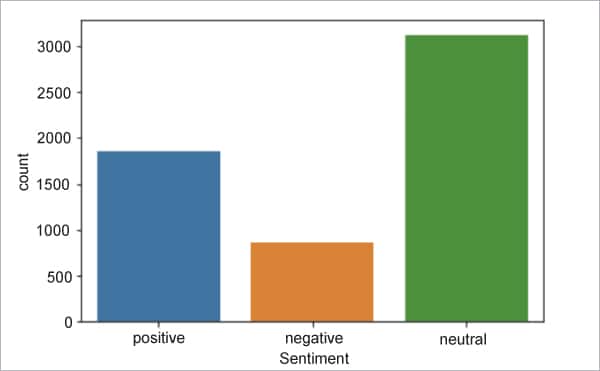
Step 3: To get an idea of how many positive, negative and neutral sentences we have in the data set, we are going to plot the data into a bar chart:

print(df[“Sentiment”].value_counts())
sns.countplot(x=”Sentiment”,data=df);

Figure 1 shows the distribution of positive, negative and neutral sentences in the data set.

Step 4: Next, we will start with cleaning and pre-processing the text before applying the MNB algorithm to boost the accuracy and precision of the training data:

stop_words = set(stopwords.words(“english”))
df[“Sentence”] = df[“Sentence”].str.replace(“\d”,””)
def cleaner(data):
    
    # Tokens
    tokens = word_tokenize(str(data).replace(“’”, “”).lower()) 
    
    # Remove Puncs
    without_punc = [w for w in tokens if w.isalpha()]
    
    # Stopwords
  without_sw = [t for t in without_punc if t not in stop_words]
    
    # Lemmatize
    text_len = [WordNetLemmatizer().lemmatize(t) for t in without_sw]
    # Stem
    text_cleaned = [PorterStemmer().stem(w) for w in text_len]
    
    return “ “.join(text_cleaned)
df[“Sentence”] = df[“Sentence”].apply(cleaner)

Step 5: Now we need to filter out the rare words that are used in the sentences.

rare_words = pd.Series(“ “.join(df[“Sentence”]).split()).value_counts()
rare_words = rare_words[rare_words <= 2]

df[“Sentence”] = df[“Sentence”].apply(lambda x: “ “.join([i for i in x.split() if i not in rare_words.index]))

Step 6: As a next step, we can generate a word cloud to see the most commonly occurring words in the text. This is an option step and more for our own understanding of the data set than anything else. Figure 2 shows the word cloud generated as a result of the code in Step 6.

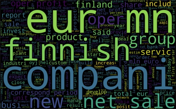
plt.figure(figsize=(16,12))
wordcloud = WordCloud(background_color=”black”,max_words=500, width=1500, height=1000).generate(‘ ‘.join(df[‘Sentence’]))
plt.imshow(wordcloud, interpolation=’bilinear’)
plt.axis(“off”)
plt.show()

Step 7: Before we execute the algorithm, we need to divide the data set into two parts. One part will be used for training the algorithm and the other for testing it.

from sklearn.model_selection import train_test_split
from sklearn.metrics import confusion_matrix,classification_report,accuracy_score
from sklearn.naive_bayes import MultinomialNB

X = df[“Sentence”]
y = df[“Target”]

X_train,X_test,y_train,y_test = train_test_split(X,y, test_size = 0.25,random_state= 42,stratify=y)

Step 8: Finally, we will execute the Multinomial Naïve Bayes algorithm on the training data:

nb_model = MultinomialNB()
nb_model.fit(X_train_count,y_train)

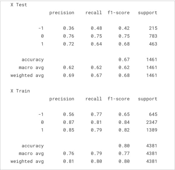
Step 9: Let us evaluate the performance of the trained MNB algorithm using the test data:

nb_pred = nb_model.predict(X_test_count)
nb_train_pred = nb_model.predict(X_train_count)
print(“X Test”)
print(classification_report(y_test,nb_pred))
print(“X Train”)
print(classification_report(y_train,nb_train_pred))

The output of the code above has been shown in Figure 3. We have successfully trained and tested the Multinomial Naïve Bayes algorithm on the data set, which can now predict the sentiment of a statement from financial news with 80 per cent accuracy.

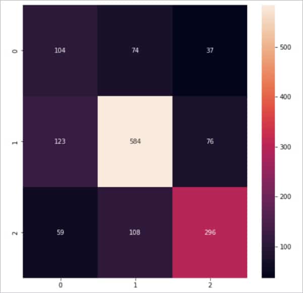
Step 10: We can visualise these results in the form of a heat map for more clarity:

plt.figure(figsize=(8,8))
sns.heatmap(confusion_matrix(y_test,nb_pred),annot = True,fmt = “d”)

Figure 4 shows the results of the MNB algorithm in the form of a heat map.

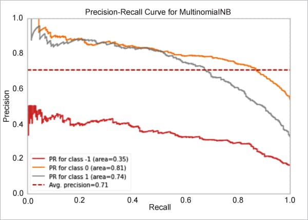
Step 11: We can also visualise these results using a precision-recall curve:

from yellowbrick.classifier import PrecisionRecallCurve
viz = PrecisionRecallCurve(MultinomialNB(),
                           classes=nb_model.classes_,
                           per_class=True,
                           cmap=”Set1”)
viz.fit(X_train_count,y_train)
viz.score(X_test_count, y_test) 
viz.show();

Figure 5 shows the precision-recall curve of the MNB algorithm.