


This sixteenth article in the R series will introduce you to correlation.
In this article, we shall explore correlation. We will use R version 4.2.1 installed on Parabola GNU/Linux-libre (x86-64) for the code snippets.
$ R --version

R version 4.2.1 (2022-06-23) -- “Funny-Looking Kid”
Copyright (C) 2022 The R Foundation for Statistical Computing Platform: x86_64-pc-linux-gnu (64-bit)

R is free software and comes with ABSOLUTELY NO WARRANTY.
You are welcome to redistribute it under the terms of the GNU General Public License versions 2 or 3.
For more information about these matters see <a href="https://www.gnu.org/licenses/." target="_blank" rel="noopener">https://www.gnu.org/licenses/.</a>
The cor() function in R can compute the correlation between two sets of vectors. Its usage is as follows:
cor(x, y, na.rm, use, method)
The correlation function accepts the following arguments:
| Argument | Description |
| x | numeric vector, matrix or data frame |
| y | vector or NULL |
| na.rm | logical value to remove missing values |
| use | string to specify the computing method |
| method | ‘pearson’, ‘kendall’, or ‘spearman’ coefficient |
Let us create three vectors ‘x’, ‘y’ and ‘z’ for comparison using the sin() and cos() functions as follows:
> t = seq(0, 10, 0.1)
> x = sin(t)
> y = sin(t + 0.05)
> z = cos(t)
The first few values of the vectors are listed below:
> head(x)
[1] 0.00000000 0.09983342 0.19866933 0.29552021 0.38941834 0.47942554

> head(y)
[1] 0.04997917 0.14943813 0.24740396 0.34289781 0.43496553 0.52268723

> head(z)
[1] 1.0000000 0.9950042 0.9800666 0.9553365 0.9210610 0.8775826
The correlation between the ‘x’ and ‘y’ vectors as well as the ‘x’ and ‘z’ vectors is shown below:
> cor(x, y)
[1] 0.9985339

> cor (x, z)
[1] 0.05483627
We observe that there is a high correlation of 0.99 between the ‘x’ and ‘y’ vectors as they come from the same sine function. The ‘x’ and ‘z’ vectors have a low correlation of 0.05 as they are defined using sine and cosine functions respectively.
Consider the mtcars data set available in the lattice library:
> head(mtcars)
mpg cyl disp hp drat wt qsec vs am gear carb
Mazda RX4 21.0 6 160 110 3.90 2.620 16.46 0 1 4 4
Mazda RX4 Wag 21.0 6 160 110 3.90 2.875 17.02 0 1 4 4
Datsun 710 22.8 4 108 93 3.85 2.320 18.61 1 1 4 1
Hornet 4 Drive 21.4 6 258 110 3.08 3.215 19.44 1 0 3 1
Hornet Sportabout 18.7 8 360 175 3.15 3.440 17.02 0 0 3 2
Valiant 18.1 6 225 105 2.76 3.460 20.22 1 0 3 1
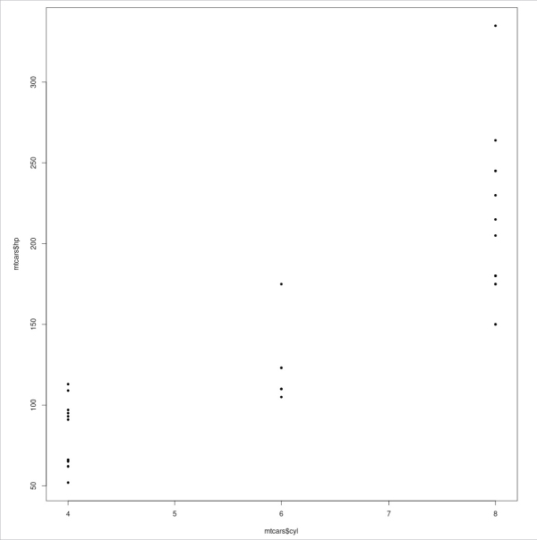
A plot comparison between cylinder size and horsepower can be generated using the plot() function, as follows:
> plot(mtcars$cyl, mtcars$hp, pch=20)
The correlation coefficient values between the cylinder size and horsepower using the default Pearson’s, Kendall’s and Spearman’s methods are given below:
> cor(mtcars$cyl, mtcars$hp)
[1] 0.8324475

> cor(mtcars$cyl, mtcars$hp, method = “kendall”)
[1] 0.7851865

> cor(mtcars$cyl, mtcars$hp, method = “spearman”)
[1] 0.9017909
The high correlation coefficient signifies that a high horsepower has a positive relation with the number of cylinders. The cor.test() function can also be used to test the association between paired samples. The correlation test between the mtcars cylinders and horsepower values is shown below:
> cor.test(mtcars$cyl, mtcars$hp)

Pearson’s product-moment correlation

data: mtcars$cyl and mtcars$hp
t = 8.2286, df = 30, p-value = 3.478e-09
alternative hypothesis: true correlation is not equal to 0
95 percent confidence interval:
0.6816016 0.9154223
sample estimates:
cor
0.8324475
The cor.test function accepts the following arguments:
| Argument | Description |
| x, y | numeric data vectors |
| alternative | ‘two.sided’, ‘greater’ or ‘less’ alternative hypothesis |
| method | ‘pearson’, ‘kendall’ or ‘spearman’ |
| exact | logical value to be indicated if exact p-value should be computed |
| conf.level | confidence level |
| continuity | true to use a continuity correction |
| data | optional data frame or matrix |
| subset | optional vector that specifies subset of observations to be used |
| na.action | function to indicate when data has NA values |
We can also handle missing values in the data source vectors by specifying the ‘use’ argument with the cor() function. An example is given below:
> a <- c(1, 3, 5)
> b <- c(2, 4, NA)

> cor(a, b)
[1] NA

> cor(a, b, use = “complete.obs”)
[1] 1
An MxN correlation matrix can be created for a data frame. For example:
> cor(mtcars)
mpg cyl disp hp drat wt
mpg 1.0000000 -0.8521620 -0.8475514 -0.7761684 0.68117191 -0.8676594
cyl -0.8521620 1.0000000 0.9020329 0.8324475 -0.69993811 0.7824958
disp -0.8475514 0.9020329 1.0000000 0.7909486 -0.71021393 0.8879799
hp -0.7761684 0.8324475 0.7909486 1.0000000 -0.44875912 0.6587479
drat 0.6811719 -0.6999381 -0.7102139 -0.4487591 1.00000000 -0.7124406
wt -0.8676594 0.7824958 0.8879799 0.6587479 -0.71244065 1.0000000
qsec 0.4186840 -0.5912421 -0.4336979 -0.7082234 0.09120476 -0.1747159
vs 0.6640389 -0.8108118 -0.7104159 -0.7230967 0.44027846 -0.5549157
am 0.5998324 -0.5226070 -0.5912270 -0.2432043 0.71271113 -0.6924953
gear 0.4802848 -0.4926866 -0.5555692 -0.1257043 0.69961013 -0.5832870
carb -0.5509251 0.5269883 0.3949769 0.7498125 -0.09078980 0.4276059

qsec vs am gear carb
mpg 0.41868403 0.6640389 0.59983243 0.4802848 -0.55092507
cyl -0.59124207 -0.8108118 -0.52260705 -0.4926866 0.52698829
disp -0.43369788 -0.7104159 -0.59122704 -0.5555692 0.39497686
hp -0.70822339 -0.7230967 -0.24320426 -0.1257043 0.74981247
drat 0.09120476 0.4402785 0.71271113 0.6996101 -0.09078980
wt -0.17471588 -0.5549157 -0.69249526 -0.5832870 0.42760594
qsec 1.00000000 0.7445354 -0.22986086 -0.2126822 -0.65624923
vs 0.74453544 1.0000000 0.16834512 0.2060233 -0.56960714
am -0.22986086 0.1683451 1.00000000 0.7940588 0.05753435
gear -0.21268223 0.2060233 0.79405876 1.0000000 0.27407284
carb -0.65624923 -0.5696071 0.05753435 0.2740728 1.00000000
The corrplot() function can be used to display a correlation matrix. You can install the same in an R session using the following command:
> install.packages(“corrplot”)

Installing package into ‘/home/guest/R/x86_64-pc-linux-gnu-library/4.1’
...
** testing if installed package can be loaded from temporary location

** testing if installed package can be loaded from final location

** testing if installed package keeps a record of temporary installation path

* DONE (corrplot)
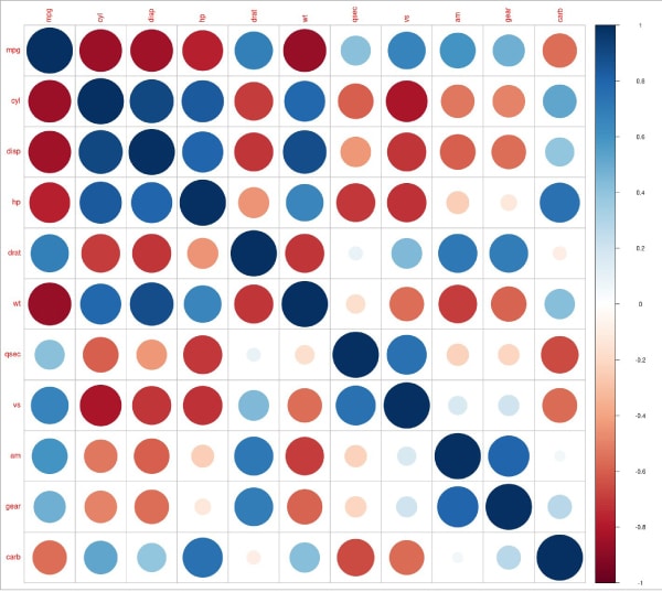
After loading the corrplot library, we can view the plot for the mtcars data set as follows:
> library(“corrplot”)
corrplot 0.92 loaded

> corrplot(cor(mtcars), method = “circle”)
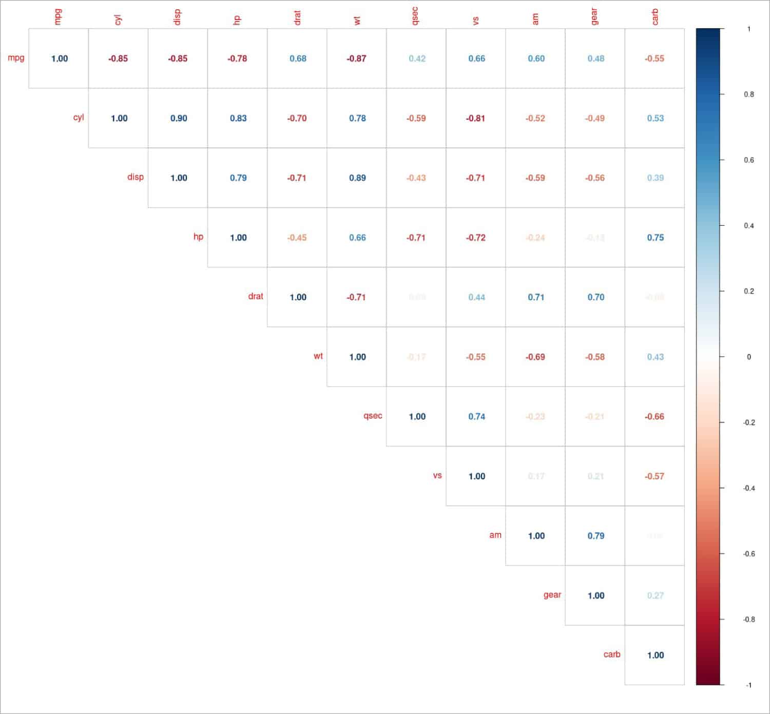
You can also restrict the plot to the upper segment by using the ‘type’ argument. For example:
> corrplot(cor(mtcars), method = “number”, type = “upper”)
The corrplot() function accepts the following arguments:
| Argument | Description |
| corr | the correlation matrix |
| method | ‘circle’, ‘square’, ‘ellipse’, ‘number’, ‘pie’, ‘shade’ and ‘colour’ |
| type | ‘full’, ‘upper’, or ‘lower’ |
| col | specifies a vector colour of glyphs |
| bg | background colour |
| title | title of the graph |
| add | logical value to add plot to an existing graph |
| diag | logical value to display the correlation coefficients |
| order | ‘original’, ‘AOE’, ‘FPC’, ‘hclust’, or ‘alphabet’ |
| rect.col | colour for the rectangular border |
| tl.cex | size of the text label |
| t1.col | colour of the text label |
| tl.srt | numeric value for text label string rotation |
Another plotting function for the correlation matrix is the ggcorplot() function, as illustrated below:
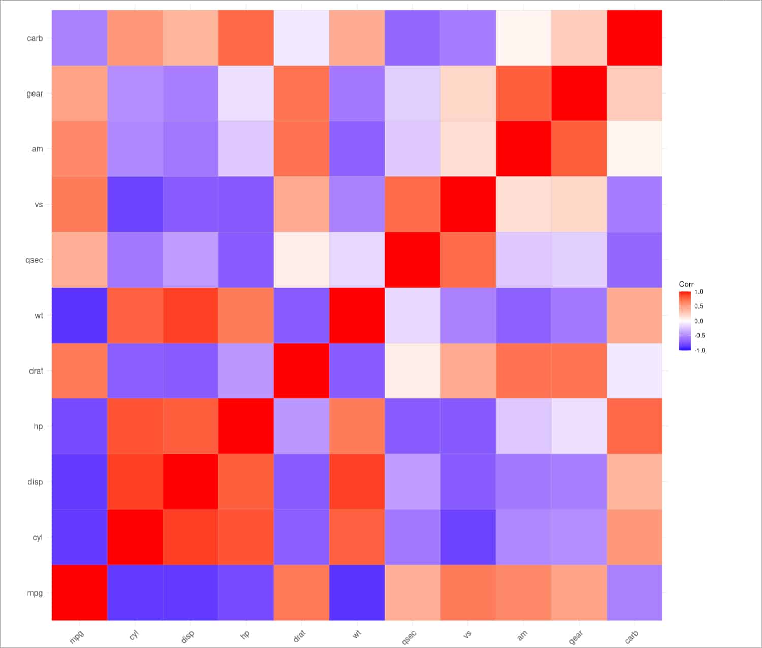
> install.packages(“ggcorrplot”)

Installing package into ‘/home/shakthi/R/x86_64-pc-linux-gnu-library/4.1’

...
** testing if installed package can be loaded from final location

** testing if installed package keeps a record of temporary installation path
* DONE (ggcorrplot)


> library(“ggcorrplot”)
Loading required package: ggplot2

> ggcorrplot(cor(mtcars))
The scatterplots are also useful for visualising the matrix. The pairs() function is used to compare the miles per gallon, displacement and horsepower, as shown below:
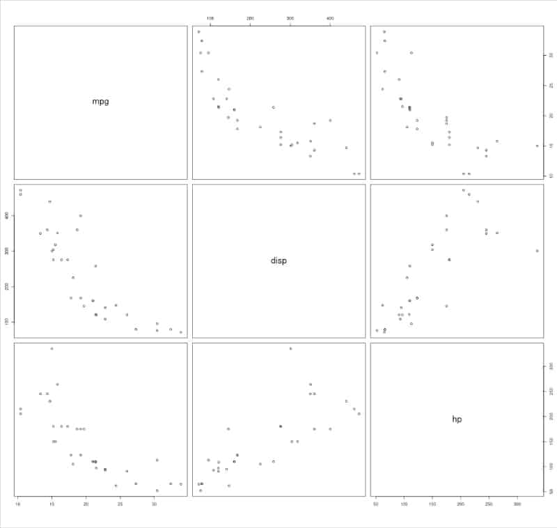
> pairs(mtcars[, c(“mpg”, “disp”, “hp”)])
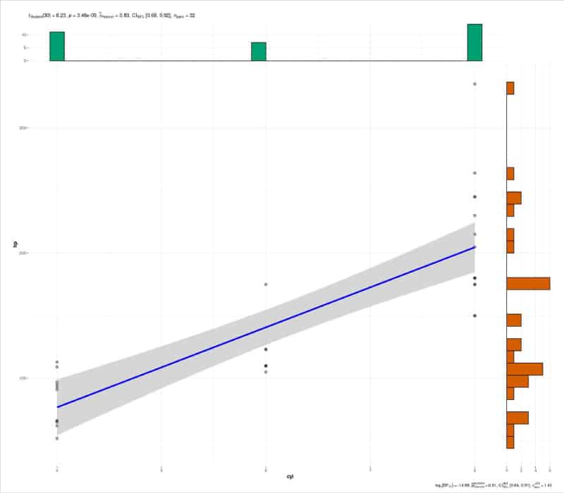
The ggscatterstats() function accepts a data frame, and produces a combined density and histogram plot. It is provided by the ggstatsplot library, which is an extension of the ggplot2 package. An example is given below:
> install.packages(“ggstatsplot”)
...
** testing if installed package keeps a record of temporary installation path

* DONE (ggstatsplot)

> library(ggstatsplot)

> ggscatterstats(data = mtcars, x = cyl, y = hp)
The ggscatterstats() function accepts the following arguments:
| Argument | Description |
| data | data frame or matrix, table, array |
| x | explanatory variable in the data |
| y | response variable in the data |
| type | ’parametric’, ’nonparametric’,’robust’,’bayes’ |
| bf.prior | prior width for calculating Bayes factors |
| bf.message | logical value to display Bayes Factor |
| tr | trim level for the mean |
| k | significant digits after decimal point |
| xfill, yfill | colour fill for x and y axes |
| xlab | label for x axis variable |
| ylab | label for y axis variable |
| title | plot title |
You are encouraged to read the manual pages for the above R functions to learn more on their arguments, options and usage.


