


This fifteenth article in the R series will explore more probability distributions and introduce statistical tests.
We will use R version 4.2.1 installed on Parabola GNU/Linux-libre (x86-64) for the code snippets.
$ R --version

R version 4.2.1 (2022-06-23) -- “Funny-Looking Kid”
Copyright (C) 2022 The R Foundation for Statistical Computing
Platform: x86_64-pc-linux-gnu (64-bit)

R is free software and comes with ABSOLUTELY NO WARRANTY.
You are welcome to redistribute it under the terms of the
GNU General Public License versions 2 or 3.
For more information about these matters see
https://www.gnu.org/licenses/.
Welch two sample t-test
Consider the mtcars data set in the lattice library:
> head(mtcars)
mpg cyl disp hp drat wt qsec vs am gear carb
Mazda RX4 21.0 6 160 110 3.90 2.620 16.46 0 1 4 4
Mazda RX4 Wag 21.0 6 160 110 3.90 2.875 17.02 0 1 4 4
Datsun 710 22.8 4 108 93 3.85 2.320 18.61 1 1 4 1
Hornet 4 Drive 21.4 6 258 110 3.08 3.215 19.44 1 0 3 1
Hornet Sportabout 18.7 8 360 175 3.15 3.440 17.02 0 0 3 2
Valiant 18.1 6 225 105 2.76 3.460 20.22 1 0 3 1
The displacement values are shown below:
> mtcars$disp
[1] 160.0 160.0 108.0 258.0 360.0 225.0 360.0 146.7 140.8 167.6 167.6 275.8
[13] 275.8 275.8 472.0 460.0 440.0 78.7 75.7 71.1 120.1 318.0 304.0 350.0
[25] 400.0 79.0 120.3 95.1 351.0 145.0 301.0 121.0
We can prepare two data sets, P and Q, from the displacement data, as follows:
> P <- mtcars$disp[0:9]
> P
[1] 160.0 160.0 108.0 258.0 360.0 225.0 360.0 146.7 140.8

> Q <- mtcars$disp[10:19]
> Q
[1] 167.6 167.6 275.8 275.8 275.8 472.0 460.0 440.0 78.7 75.7
The boxplot for the data sets is shown in Figure 1:
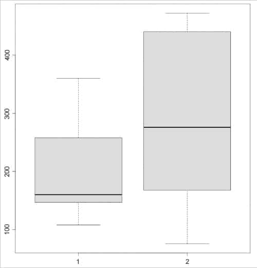
> boxplot(P, Q)
The Welch two sample t-test can be performed using the t.test() function, as demonstrated below:
> t.test(P, Q)

	Welch Two Sample t-test

data:  P and Q
t = -0.98055, df = 15.369, p-value = 0.342
alternative hypothesis: true difference in means is not equal to 0
95 percent confidence interval:
 -176.63004   65.16337
sample estimates:
mean of x mean of y
 213.1667  268.9000
We can also run the t-test assuming equal variances by passing TRUE to the ‘var.equal’ argument, as follows:
> t.test(P, Q, var.equal=TRUE)

	Two Sample t-test

data:  P and Q
t = -0.95746, df = 17, p-value = 0.3518
alternative hypothesis: true difference in means is not equal to 0
95 percent confidence interval:
 -178.54460   67.07793
sample estimates:
mean of x mean of y
 213.1667  268.9000
Two sample Wilcoxon test
The Mann-Whitney-Wilcoxon test is used for randomly selected values from two populations. For our example, we can run the wilcox.test() function on the P and Q data sets, as follows:
> wilcox.test(P, Q)

	Wilcoxon rank sum test with continuity correction

data:  P and Q
W = 32, p-value = 0.3059
alternative hypothesis: true location shift is not equal to 0

Warning message:
In wilcox.test.default(P, Q) : cannot compute exact p-value with ties
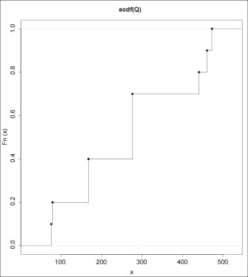
The empirical CDFs for the data sets can be drawn using the plot() function:
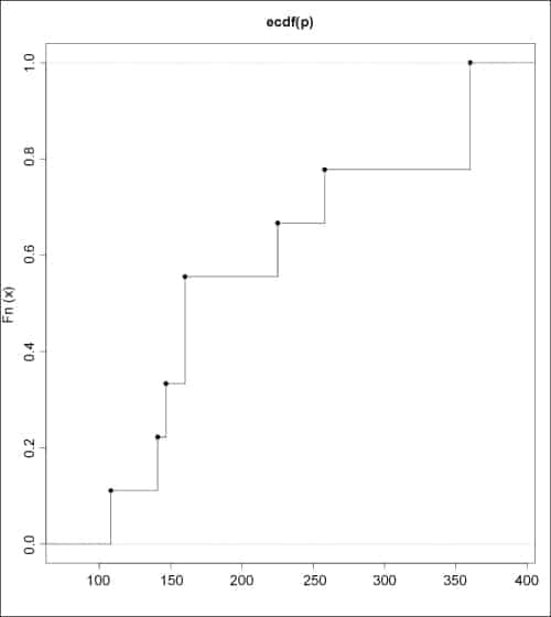
> plot (ecdf(P), verticals=TRUE)
> plot (ecdf(Q), verticals=TRUE)
The wilcox.test() function accepts the following arguments:
| Arguments | Description |
| x | A numeric vector of data values |
| y | Optional numeric vector of data values |
| alternative | Character string for alternative hypothesis (‘two.sided’, ‘greater’, or ‘less’) |
| conf.int | A logical value that indicates if confidence interval should be computed |
| conf.level | Confidence level of the interval |
| correct | A logical value on whether to apply continuity correction |
| data | An optional matrix or data frame |
| exact | A logical value on whether p-value should be computed |
| mu | Optional parameter for the null hypothesis |
| na.action | A function to handle data that contains NAs |
| paired | A logical value to indicate a paired test |
| subset | An optional vector specifying a subset of observations |
| tol.root | A positive numeric tolerance |
Kolmogrov-Smirnov test
The Kolmogrov-Smirnov test or KS test is used to test if two samples come from the same distribution. It can also be modified to be used as a ‘goodness of fit’ test. The two-sample Kolmogrov-Smirnov test for the P and Q data sets is as follows:
> ks.test(P, Q)

	Exact two-sample Kolmogorov-Smirnov test

data:  P and Q
D = 0.37778, p-value = 0.2634
alternative hypothesis: two-sided
You can also perform a one-sample Kolmogrov-Smirnov test. The function accepts the following arguments:
| Arguments | Description |
| x | Numeric vector of data values |
| y | Numeric vector or character string name of a CDF |
| alternative | Alternate hypothesis should be ‘two-sided’, ‘less’ or ‘greater’ |
| exact | NULL or logical value to specify if p-value should be computed |
| simulate.p.value | A logical value to compute p-values by Monte Carlo simulation |
| data | An optional data frame |
| subset | A subset vector of data to be used |
| na.action | A function to handle data that contains NAs |
The alternative hypothesis argument accepts the string argument values: ‘two.sided’, ‘less’, and ‘greater’. These indicate if the null hypothesis of the distribution of ‘x’ is equal to, less than, or greater than the distribution of ‘y’. Any missing values are ignored from both the samples.
Chi-Square test
The Chi-Square test is a statistical hypothesis test to determine the correlation between two categorical variables. We can determine if the cylinder and horse power variables from the mtcars data set are significantly correlated.
> data <- table(mtcars$cyl, mtcars$hp)
> print(data)

    52 62 65 66 91 93 95 97 105 109 110 113 123 150 175 180 205 215 230 245 264
  4  1  1  1  2  1  1  1  1   0   1   0   1   0   0   0   0   0   0   0   0   0
  6  0  0  0  0  0  0  0  0   1   0   3   0   2   0   1   0   0   0   0   0   0
  8  0  0  0  0  0  0  0  0   0   0   0   0   0   2   2   3   1   1   1   2   1
The chisq.test() function can be performed on the data variables, as shown below:
> chisq.test(data)

	Pearson’s Chi-squared test

data:  data
X-squared = 59.429, df = 42, p-value = 0.0393
A p-value of less than 0.05 shows that there is a strong correlation between cylinder and horsepower.
The chisq.test function accepts the following arguments:
| Arguments | Description |
| x | A numeric vector or matrix |
| y | A numeric vector, or ignored by x is a matrix |
| correct | A logical value on whether to apply continuity correction |
| p | A vector of probabilities |
| rescale.p | A logical scalar to sum to 1 |
| simulate.p.value | A logical value to whether compute p-values by Monte Carlo simulation |
Beta
The Beta function is mathematically defined by the integral for two inputs, alpha and beta, as shown below:

You can use the beta() function for the P and Q data sets, as follows:
> beta(P, Q)
 [1] 7.307338e-100 7.307338e-100 2.515827e-100 5.970038e-162 2.168131e-190
 [6] 8.246568e-192 1.139582e-245 1.211659e-144  2.186038e-63  1.931142e-65
The lbeta() function provides the natural logarithm of the beta function, as demonstrated below:
> lbeta(P, Q)
 [1] -228.2696 -228.2696 -229.3359 -371.2320 -436.7173 -439.9865 -564.0027
 [8] -331.3803 -144.2808 -149.0099
The dbeta() function provides the density distribution. An example is given below with a plot (Figure 5).
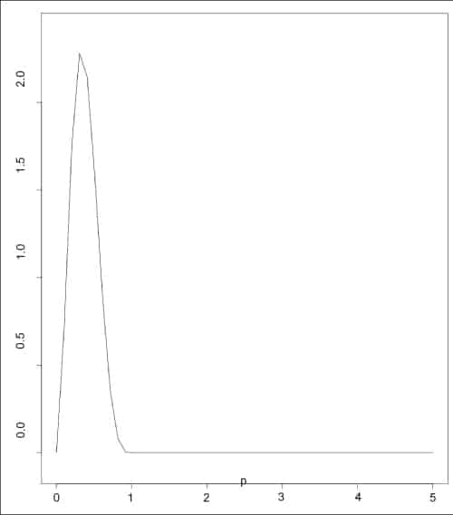
> p = seq(0, 5, length=50)
> plot(p, dbeta(p, 3, 5), type=’l’)
Gamma
The Gamma distribution is a continuous probability distribution that has a shape (z) and scale parameter (k), which is defined as shown in Figure 6.
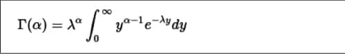
The dgamma() function provides the density function. In the following example, a sequence of values is produced and a plot for its gamma distribution is generated.
> a <- seq(0, 50, by=0.01)
> y <- dgamma(a, shape=3)
> plot(y)
The lgamma() function provides the natural logarithm of the absolute value of the gamma function. For example:
> l <- lgamma(a)
> head(l)
[1] Inf 4.599480 3.900805 3.489971 3.197078 2.968879
These functions accept the following arguments:
| Arguments | Description |
| a, b | Positive numeric vectors |
| x, n | Numeric vectors |
| k, d | Integer vectors |


