


")
Cache is a crucial strategy for improving system performance as it temporarily stores data for quick retrieval, preventing the need to read from the original data source repeatedly, which can be time consuming. Several algorithms have been developed to increase the cache hit ratio. Some of these are discussed here.
In general, caching is used by operating systems, CPUs, GPUs, web browsers, applications, CDNs (content delivery networks), DNS (domain name systems), databases, and even at the ISP (internet service provider) level.
Before delving into a detailed discussion on cache, let’s clarify some concepts often confused with it.
Caching vs buffering vs streaming vs register vs cookies
Caching: Storing partial or small data for quick retrieval
Buffering: Using a buffer to store data when there is a difference in the speed and processing of data between the sender and receiver
Streaming: Real-time data broadcasting, whether audio, video, or text
Register: Very small memory storage in computer processors for fast retrieval by the processor; typically stores data that the CPUs are processing
Cookies: Used in web browsers to maintain small data holding user preferences or login details, and is quite different from caching
We will see the various techniques used to save particular data temporarily, as we cannot save the entire stuff. Caching techniques can be used in different systems, such as:
- Cache memory
- Cache servers
- CPU cache
- Disk cache
- Flash cache
- Persistent cache
Cache is considered effective when the client requests data and it hits the cache rather than reading from the direct memory — this is termed as cache hit, else it’s a cache miss. Several algorithms are used to increase the cache hit ratio based on application requirements. A few are briefly described below.
Cache algorithms
Spatial
- This caching technique is used to perform advanced reads of the nearest data from the recently used data.
- The idea behind reading closely associated data is it increases the chances of reading this data as well.
- This will increase the performance as the manual read is avoided and the data is ready to be served.
- For example, data saved in an array or similar type of records from a table can be read with a single read instruction from the original source and saved in the cache. This avoids multiple iterations of read requests.
FIFO (first in first out)
- Data is added to the queue as it is accessed.
- Once the cache is full, the first added item is removed from the cache.
- The ejection occurs from the order of data being added.
- From the point of view of the terms of implementation and performance this technique is fast but not smart.
LIFO (last in first out)
- This is the opposite of FIFO — once the cache is full, the last added item is removed first.
- The ejection occurs in the reverse of the order of data being added.
- This technique, too, is fast but not smart.
LFU (least frequently used)
- Here the data keeps track of how frequently it has been used from the cache, and the count is maintained.
- Once the cache is full, the lowest count data gets removed first.
LRU (least recently used)
- Initially any read data is added to the cache, but when the cache is full it frees up the least recently used data.
- Here, each time the data is read from the cache it’s moved to the top of the queue, increasing its significance.
- This is a fast and most commonly used algorithm.
- ‘Temporal Locality’ uses a similar concept while saving the recently used instructions in cache memory, as there are high chances of these being used again.
LRU2 (least recently used twice)
- Two caches are maintained here — the item is added to the main cache only when it is accessed a second time.
- Once the cache is full, the least recently accessed item is removed.
- This is complex and more space is required, as there are two caches and the count of accesses is maintained.
- The advantage is the main cache holds the most frequently and recently accessed data.
2Q (two queue)
- Here, as well, two queues — one small and one large — are maintained.
- First, accessed data is added to the smaller LRU queue.
- If the same data is accessed a second time, it is moved to the larger LRU and removed from the first queue.
- Performs better than LRU2 and makes it adaptive.
MRU (most recently used)
- Quite opposite to LRU, here the most recently accessed data is removed from the cache.
- This algorithm leans towards the older data, which is more likely to be used again.
STBE (simple time based expiration)
- Here, once the data is added to the cache, its lifetime tickers get started.
- Data is removed from the cache after a certain time period, e.g., at 5.00 pm or a particular date or time.
ETBE (extended time based expiration)
- Data from the cache is removed after a certain time period.
- Here the time to evict data is configurable; e.g., five hours from now, or every ten minutes.
SLTBE (sliding time based expiration)
- The timeline of the data extends after being accessed from the cache.
- In this algorithm, the most recently accessed data gets more time to stay in the cache.
WS (working set)
This is similar to LRU, but here a flag is created for each access in the cache.
- Periodically, the cache is checked, considering the recently accessed data in the working sets.
- Non-working set data is removed when the cache is full.
RR (random replacement)
- Here, data is picked randomly from the cache and replaced with the newly accessed data.
- This approach does not keep track of the history, resulting in less overhead, but the results are not guaranteed.
LLF (lowest latency first)
- This algorithm keeps track of download latency time.
- The data with the least downloaded latency time is evicted first, as it can be quickly retrieved again.
- Here, the advantage is when complex data needs to be retrieved, it can be easily referred from the cache.
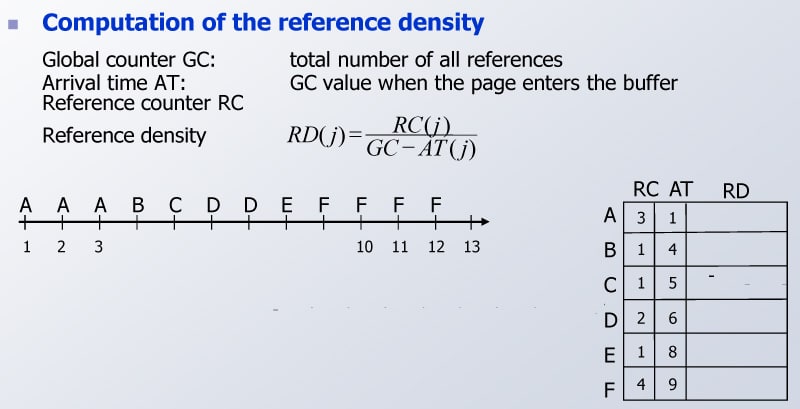
LRD (least reference density)
- The object with the least reference density is removed when the cache is full.
- A global reference counter is maintained, containing the sum of all references in the cache.
- The reference density (RD) is calculated based on:
- Object’s reference counter (RC) meaning the number of times it has been accessed
- Total number of all the references (GC)
- Each object has an arrival timestamp (AT), which is the current GC value when it’s been added to the cache
- The reference density (RD) is computed as the ratio between the object’s reference counter (RC) and the number of references added since the object was included into the cache (GC – AT):
- RC(i) / (GC – AT(i)).
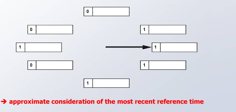
Clock
- Clock is an efficient version of FIFO, where data in the cache does not have to be constantly pushed to the back of the list but performs a general function as ‘Second Chance’ in a circular queue.
- ‘Second Chance’ is a bit assigned to each object data in the cache, and it is set to be 1 when it has been referenced, giving it a second chance.
- During the eviction operation, the object follows the FIFO queue, but to be evicted, the object needs to be 0. So, if in the queue the object was recently accessed it would have been ‘1’, though after the eviction the flag is reset to 0 again.
- Thus the data gets a second chance of not being replaced during its first consideration.
GCLOCK (generalised clock)
- This is a mix between LFU (last frequently used) and LRU (last recently used) replacement policies.
- The reference counts are used to track references to cached objects.
- Each access request increments the reference count
of the object. - If the cache is full, the object to be removed is determined by decrementing the reference count for each object.
- After decrement, an object is replaced by the object in which reference count = 0 is found.
- This implementation tends to replace younger
objects first.
ARC (adaptive replacement cache)
- ARC dynamically balances recency and frequency using a set of rules, and performs self-tuning.
- It keeps track of recently and frequently accessed data queues, along with the entries of recently and frequently removed data, also called ghost entries.
- These entries help the algorithm to expand or shrink the LRU or LFU, based on the usage.
- ARC enables substantial performance gains over commonly used modules.
- There is another variant of ARC — SARC or sequential prefetching in adaptive replacement cache — which is claimed to be better.
DeepBM
- This is a deep learning-based dynamic page replacement policy (https://people.eecs.berkeley.edu/~kubitron/courses/cs262a-F18/projects/reports/project16_report.pdf).
- Using deep learning, this algorithm learns from the past and dynamically adapts to the workload, which predicts the page to be evicted from the cache.
Cache policies
Cache policies determine how the cache operates in terms of writes to the storage.
- Write around cache
- Writes to the storage first and skips the cache.
- Here the advantage is when there is a large amount of write, the cache will not need to be overloaded with write I/O.
- But there are two common problems — data could be stale in the cache, and reads could be slower as the new data will not be present in the cache.
- Write through cache
- Write is performed in the system, cache, and actual storage.
- The advantage here is reads will be faster as the most recently written data is available in the cache.
- But write will be slower as it needs to wait until the write is successful in both the systems.
- Write back cache
- Write operation takes place in the cache first, and is considered to be completed if the data is written to the cache.
- From here, the data is copied back to the storage.
- In this case, both the read and write could be faster.
- But the greatest challenge is inconsistent writes, as there is a possibility of not being written to persistent storage.
Pros and cons of caching
Pros
- Performance improvement is expected if the right cache algorithm is used.
- Can act as middleware when the connectivity is lost, allowing offline operations to sync once the system is online.
Cons
- Performance can be impacted if the cache ratio is low.
- Invalid or outdated information could result in misinformation, and there is a need to take special care that data in cache is not stale.
New caching techniques and algorithms are being continuously developed, but for now we have explored a few that can help better system performance. In conclusion, a quote to remember in the context of this article: “There are only two hard things in computer science: cache invalidation and naming things.” — Phil Karlton


