


Julia is a programming language that produces code which runs considerably faster than its counterparts. This article introduces JuliaDB – an analytical database that is entirely created in Julia. The various advantages of JuliaDB include JIT compilation, powerful parallelism and a super-fast CSV parser. So let’s explore JuliaDB further.
Julia is a powerful programming language. The programming languages can be broadly grouped into two categories — those that are easy to build programs with but the code created runs comparatively slower (e.g., Python), and those with which building programs requires more time but the resultant code runs considerably faster (e.g., C++). Julia is aimed at combining the benefits of both these programming worlds. If you are new to Julia, there have been earlier articles (five, to be precise) on the subject in Open Source For You itself, which can be referred to at https://www.opensourceforu.com/?s=Julia.
JuliaDB is an analytical database. When compared with similar options such as Pandas, the features provided by JuliaDB are better. At the same time, JuliaDB is also comparatively faster.
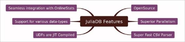
The major features of JuliaDB are listed below:
- Just-in-time compilation
- Superior parallelism
- It can store many types of data.
- The UDF (user defined functions) are faster, as they are also JIT compiled.
- It has a super-fast CSV parser that can handle large files without a lag.
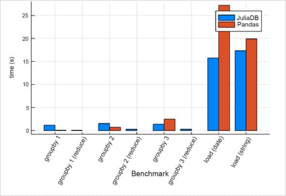
Comparing the performance of JuliaDB with other analytical databases
As per the official website of JuliaDB, the performance with respect to large CSV files is better. Figure 2 shows a comparison between JuliaDB and Pandas (source: https://juliadb.org/ ).
The design goals of JuliaDB are as follows:
- To have the capability to load multi-dimensional data sets faster with incremental support.
- The capability to index data and perform tasks such as aggregate, sort, filter and join.
- The capability to store the results and load them when required in a faster and more efficient way.
- The capability to use the parallelism to the maximum extent possible.
| Feature | JuliaDB | Pandas | xts | TimeArrays |
| Distributed computing | Yes | – | – | – |
| Data larger than memory | Yes | – | – | – |
| Multiple indexes | Yes | – | – | – |
| Index type(s) | Any | Built-ins | Time | Time |
| Value type(s) | Any | Built-ins | Built-ins | Any |
| Compiled UDFs | Yes | – | – | Yes |
JuliaDB is built as an analytical database tool with all of the objectives mentioned earlier. The greatest advantage of JuliaDB is that it has been built all along in Julia itself, giving users the ability to compose queries with Julia code.
The fundamental components of JuliaDB are IndexedTable and NDParse data structures. Typed columns based storage makes the aggregation operations very fast.
Getting started with JuliaDB
Similar to any other package in Julia, JuliaDB can be added to your system with the following commands:
using Pkg
Pkg.add(“JuliaDB”)

using JuliaDB
A simple way to build a table is to use the following command:
t = table(rand(Bool, 10), rand(10))
A sample output is as shown below:
julia> t = table(rand(Bool, 10), rand(10))
Table with 10 rows, 2 columns:
1 2
───────────────
true 0.94025
true 0.99059
false 0.135366
true 0.201484
true 0.454071
true 0.462337
false 0.299111
true 0.73977
true 0.485396
false 0.169812
Here, two columns have been built. The first column carries a Boolean value and the second one a random number.
Getting and loading data
As previously stated, JuliaDB is very good at handling CSV files. You can download the hflights.csv from https://raw.githubusercontent.com/piever/JuliaDBTutorial/master/hflights.csv. Many examples in this article are based on this CSV file.
This CSV can be loaded with the following code snippet:
using JuliaDB
flights = loadtable(“hflights.csv”)
On successful loading of this table, you will get an output as shown in Figure 3.
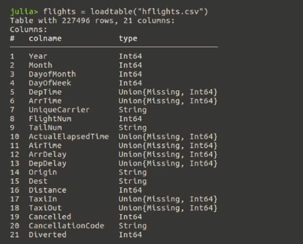
It lists all the 21 columns and their data types.
Extracting data matching a condition
The rows that meet a particular condition can be extracted with the filter function. A sample filter function is shown below:
filter(i -> (i.Month == 10) && (i.DayofMonth == 22), flights)
Obviously, this function matches rows where the month is 10 and DayofMonth is 22. You can combine conditions as shown below:
filter(i -> (i.UniqueCarrier == “AA”) || (i.UniqueCarrier == “UA”), flights)
Selecting specific columns
Specific columns can be selected with column names. A sample Select function and its output are shown below:
julia> select(flights, (:FlightNum, :Origin, :Dest))
Table with 227496 rows, 3 columns:
FlightNum Origin Dest
──────────────────
428 “IAH” “DFW”
428 “IAH” “DFW”
428 “IAH” “DFW”
428 “IAH” “DFW”
428 “IAH” “DFW”
428 “IAH” “DFW”
428 “IAH” “DFW”
428 “IAH” “DFW”
428 “IAH” “DFW”
428 “IAH” “DFW”
428 “IAH” “DFW”
428 “IAH” “DFW”
428 “IAH” “DFW”
⋮
1231 “HOU” “SAT”
124 “HOU” “STL”
280 “HOU” “STL”
782 “HOU” “STL”
1050 “HOU” “STL”
201 “HOU” “TPA”
471 “HOU” “TPA”
1191 “HOU” “TPA”
1674 “HOU” “TPA”
127 “HOU” “TUL”
621 “HOU” “TUL”
1597 “HOU” “TUL”
Nesting and piping
When you want to carry out multiple operations one after another, it can be done in two ways — by nesting and/or piping.
In the following code snippet, we are nesting by filtering for departure delays of more than 40 (!ismissing is used to detect missing values and select two columns).
filter(i -> !ismissing(i.DepDelay > 40), select(flights, (:UniqueCarrier, :DepDelay)))
Piping can be achieved with the Lazy package.
import Lazy
Lazy.@as x flights begin
select(x, (:UniqueCarrier, :DepDelay))
filter(i -> !ismissing(i.DepDelay > 60), x)
end
Sorting
Sorting can be carried out with the Sort function, as shown below:
julia> sort(flights, :FlightNum, select = (:FlightNum, :Origin, :Dest))
Table with 227496 rows, 3 columns:
FlightNum Origin Dest

────────────────────────
1 “IAH” “HNL”
1 “IAH” “HNL”
1 “IAH” “HNL”
1 “IAH” “HNL”
1 “IAH” “HNL”
1 “IAH” “HNL”
1 “IAH” “HNL”
1 “IAH” “HNL”
1 “IAH” “HNL”
1 “IAH” “HNL”
1 “IAH” “HNL”
1 “IAH” “HNL”
1 “IAH” “HNL”
⋮
7037 “IAH” “IAD”
7037 “IAH” “IAD”
7037 “IAH” “IAD”
7037 “IAH” “IAD”
7037 “IAH” “IAD”
7231 “IAH” “IAD”
7240 “IAH” “IAD”
7240 “IAH” “IAD”
7240 “IAH” “IAD”
7240 “IAH” “IAD”
7290 “IAH” “IAD”
7290 “IAH” “IAD”
Row-wise operations
You can use map() to apply some operations to every row. In the following example, the distance is divided by airtime and it’s multiplied by 60.
speed = map(i -> i.Distance / i.AirTime * 60, flights)
Adding a new column
A new column can be added to the existing data set with the help of the transform function:
flights = transform(flights, :Speed => speed)
This adds ‘Speed’ as the 22nd column to the existing flight’s data set.
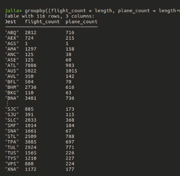
Let us suppose that for each destination, you want to find the count of the total flights and the number of distinct planes. This can be achieved with a groupby as shown below:
groupby((flight_count = length, plane_count = length∘union), flights, :Dest, select = :TailNum)
The output is shown in Figure 4.
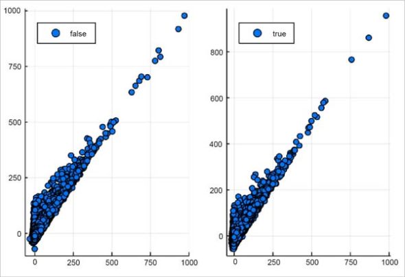
Visualisation
One of the greatest advantages of Julia is the availability of professional grade visualisation packages, an example of which is shown below:
using StatsPlots
gr(fmt = :png) # choose the fast GR backend
@df flights scatter(:DepDelay, :ArrDelay, group = :Distance .> 1000, layout = 2, legend = :topleft)
OnlineStats
OnlineStats is a popular package to compute statistics, one observation at a time. It is based on the parallel algorithms. OnlineStats can be integrated with JuliaDB in a seamless manner. Its biggest advantage is that it can handle streaming and Big Data that does not fit in memory. Figure 6 illustrates the computation of statistics in parallel, in JuliaDB.
Integration of OnlineStats is facilitated with reduce() and groupreduce(). Code examples are as shown below:
julia> using JuliaDB, OnlineStats

julia> t = table(1:100, rand(Bool, 100), randn(100));

julia> reduce(Mean(), t; select = 3)
Mean: n=100 | value=-0.0439736
For groupreduce(), the code is:
julia> grp = groupreduce(Mean(), t, 2; select=3)
Table with 2 rows, 2 columns:
1 2
───────────────────

false Mean: n=42 | value=-0.0488427
true Mean: n=58 | value=-0.0404477
To summarise, JuliaDB has various features to process data. With the inherent speed advantage of Julia and the support for parallelism, JuliaDB’s performance is superior to that of its counterparts. If you are a data science enthusiast, you may find JuliaDB very useful.


