By mastering the art of upsampling and downsampling, we not only correct skewed datasets but also pave the way for fairer, more accurate machine learning models. This first article in the two-part series focuses on the uses of upsampling.

We rely on history for future predictions, but in reality, historical data may not be sufficiently representative for accurate forecasting. As an example, historically, most top-level executive positions have been occupied by men. However, it is crucial to ensure that women who are qualified and come from diverse backgrounds are also afforded equal opportunities. Another illustration of imbalance lies in loan applications, where approximately 90% are typically rejected and only 10% are approved. This skewed ratio can lead to erroneous decisions, resulting in good loan applications being unfairly rejected. Utilising such imbalanced data for model learning can yield biased outputs supporting the majority class in predictions. Numerous real-world scenarios exhibit such data imbalances.

Another factor contributing to biased outcomes is the method of data collection. Sampling, a data collection technique involving a small subset of the population, often introduces imbalance, yielding biased data.

To counter such imbalanced datasets, we use techniques called upsampling and downsampling.

Upsampling

Upsampling involves augmenting the number of instances in a dataset and is particularly useful when there is an imbalanced distribution of data, with one class significantly underrepresented. This process involves generating synthetic data points using different techniques or generative models akin to the existing data and integrating them into the dataset. However, it is important to guard against overfitting by ensuring that the addition of new data doesn’t adversely affect the model. Following this process, the count of the classes is almost balanced.

Methods used in upsampling

Upsampling is applicable in scenarios where the dataset exhibits an imbalanced distribution or is relatively small. One effective technique for addressing class imbalance in machine learning is oversampling, wherein the minority class is oversampled by duplicating its examples in the training dataset before fitting the model. While this rebalances the class distribution, it doesn’t offer any new information to the model. Upsampling can enhance model performance, particularly in identifying rare events or anomalies. It is worth noting that the methods explained below are not exhaustive, but offer practical insights.

Resample

• Resample upsamples a dataset by simply duplicating records from minority classes.
• Logic
  • The default strategy involves executing the bootstrapping procedure.
  • Bootstrapping entails creating subsets from a dataset multiple times.
  • Depending on the size chosen, it basically creates a random selection with or without replacement of the dataset.
    • Sampling without replacement: A subset of observations is randomly selected, and once an observation is chosen, it cannot be selected again.
    • Sampling with replacement: A subset of observations is randomly selected, and an observation may be chosen multiple times.
  • The resample function is specifically used to resample a dataset n_samples times, with the default option being to sample with replacement.
• Sample code is given below:

from collections import Counter
from sklearn.datasets import make_classification
from sklearn.utils import resample
from matplotlib import pyplot
from numpy import where
import pandas as pd
import numpy as np

X, y = make_classification(n_classes=2, class_sep=2,
weights=[0.1, 0.9], n_features=4, n_clusters_per_class=1, n_samples=1000, random_state=10)

# summarize class distribution
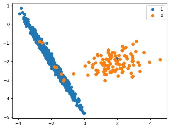
print(‘Original dataset shape %s’ % Counter(y))
Original dataset shape Counter({1: 894, 0: 106})

# scatter plot of examples by class label
for label, _ in Counter(y).items():
row_ix = where(y == label)[0]
pyplot.scatter(X[row_ix, 0], X[row_ix, 1], label=str(label))

In this code we will see how upsampling is done:

df = pd.DataFrame(X, columns=[‘Column_A’, ‘Column_B’, ‘Column_C’, ‘Column_D’])
df[‘Y’] = y
over_samples = df[df[“Y”] == 1]
under_samples = df[df[“Y”] == 0]
print(“Original Under Sample Shape”, under_samples.shape)
df_res = resample(under_samples,
replace=True,
n_samples=len(over_samples),
random_state=42)
print(“Resampled Under Sample Shape”, df_res.shape)

X_Res = np.append(df_res[[‘Column_A’, ‘Column_B’, ‘Column_C’, ‘Column_D’]].to_numpy(), over_samples[[‘Column_A’, ‘Column_B’, ‘Column_C’, ‘Column_D’]].to_numpy(), axis=0)
y_res = np.append(df_res[‘Y’].to_numpy(), over_samples[‘Y’].to_numpy())

print(‘Resampled dataset shape %s’ % Counter(y_res))
Original Under Sample Shape (106, 5)
Resampled Under Sample Shape (894, 5)
Resampled dataset shape Counter({0: 894, 1: 894})

# scatter plot of examples by class label
for label, _ in Counter(y_res).items():
row_ix = where(y_res == label)[0]
pyplot.scatter(X_Res[row_ix, 0], X_Res[row_ix, 1], label=str(label))

RandomOverSampler

• Here we randomly select the rows from the minority class and perform duplication.
• Logic
  • Random oversampling involves duplicating examples from the minority class and adding them to the training dataset.
  • This is done by making exact copies of the minority class examples, which are selected randomly with replacement from the training dataset.
• The source code is:

from collections import Counter
from sklearn.datasets import make_classification
from imblearn.over_sampling import RandomOverSampler
from matplotlib import pyplot
from numpy import where

X, y = make_classification(n_classes=2, class_sep=2,
weights=[0.1, 0.9], n_features=4, n_clusters_per_class=1, n_samples=1000, random_state=10)

# summarise class distribution
print(‘Original dataset shape %s’ % Counter(y))
Original dataset shape Counter({1: 894, 0: 106})

Now let us see how upsampling is performed:

ros = RandomOverSampler(random_state=24)
X_Res, y_res = ros.fit_resample(X, y)
print(‘Resampled dataset shape %s’ % Counter(y_res))
Resampled dataset shape Counter({1: 894, 0: 894})

# scatter plot of examples by class label
for label, _ in Counter(y_res).items():
row_ix = where(y_res == label)[0]
pyplot.scatter(X_Res[row_ix, 0], X_Res[row_ix, 1], label=str(label))
pyplot.legend()
pyplot.show()

SMOTE (Synthetic Minority Oversampling Technique)

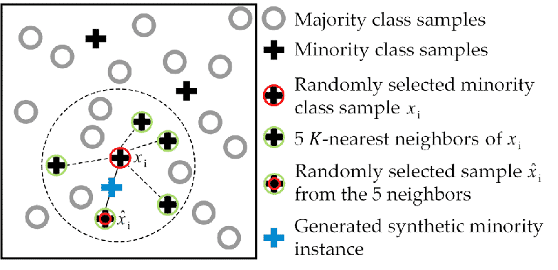
• SMOTE is a widely used method for creating new examples. It involves selecting examples that are similar in the feature space, drawing a line between them, and generating a new sample at a point along that line.
• Logic
  • It works based on the K Nearest Neighbours algorithm, by generating the synthetic data points that fall under the existing minority class.
  • To be more specific, SMOTE randomly selects an instance from the minority class and identifies its k nearest minority class neighbours (usually k=5). Then, it randomly selects a neighbour from the k nearest neighbours, and creates a synthetic example at a randomly chosen point between the two examples in the feature space.
  • To generate the synthetic instances, SMOTE uses a convex combination of the two selected instances, a and b, which are connected by a line segment in the feature space.
  • Input records should not contain null values.
• Visualisation is shown in Figure 4.

• The source code is:

from collections import Counter
from sklearn.datasets import make_classification
from imblearn.over_sampling import SMOTE
from matplotlib import pyplot
from numpy import where

X, y = make_classification(n_classes=2, class_sep=2,
weights=[0.1, 0.9], n_features=4, n_clusters_per_class=1, n_samples=1000, random_state=10)

# summarize class distribution
print(‘Original dataset shape %s’ % Counter(y))
Original dataset shape Counter({1: 894, 0: 106})

# perform upsampling
sm = SMOTE(random_state=42)
X_res, y_res = sm.fit_resample(X, y)
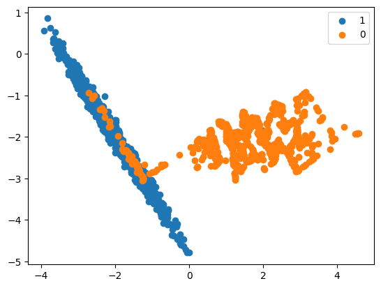
print(‘Resampled dataset shape %s’ % Counter(y_res))
Resampled dataset shape Counter({1: 894, 0: 894})

# scatter plot of examples by class label post upsampling
for label, _ in Counter(y_res).items():
row_ix = where(y_res == label)[0]
pyplot.scatter(X_res[row_ix, 0], X_res[row_ix, 1], label=str(label))
pyplot.legend()
pyplot.show()

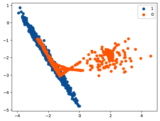
ADASYN (Adaptive Synthetic)

• Oversampling can be done using the Adaptive Synthetic (ADASYN) algorithm. This algorithm works similarly to SMOTE (can be considered as an extension), but it generates a varying number of samples based on the local distribution of the class that needs to be oversampled.
• Logic
  • ADASYN is a technique that generates synthetic samples for minority classes using the feature space of the original dataset. It calculates the density distribution of each minority class sample and generates synthetic samples according to the density distribution. The main idea behind ADASYN is to use a weighted distribution for different minority class examples based on their level of difficulty in learning. It generates more synthetic data for minority class examples that are harder to learn compared to those that are easier to learn.
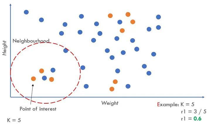
  • Randomly selects an instance from the minority class and identifies its k nearest minority class neighbours (usually k=5).
  • Finds the ratio ri = majority_class in neighbourhood / K.
  • The ri value indicates the dominance of the majority class in each specific neighbourhood. Higher ri neighbourhoods contain more majority-class examples and are more difficult to learn.

• Because ri is higher for neighbourhoods dominated by majority class examples, more synthetic minority class examples will be generated for those neighbourhoods. This is what gives the ADASYN algorithm its adaptive nature, generating more data for harder-to-learn neighbourhoods.
  • The main difference between ADASYN and SMOTE is that ADASYN generates synthetic samples adaptively based on the density distribution of minority class samples, while SMOTE generates synthetic samples by interpolating between minority class samples. This adaptive approach helps to focus more on difficult-to-learn samples, potentially leading to better classification performance.
  • However, ADASYN has a limitation of increased computational complexity due to the generation of synthetic samples. This may affect the training time of machine learning models.
• Visualisation is shown in Figure 6.

• The sample code is:

from collections import Counter
from sklearn.datasets import make_classification
from imblearn.over_sampling import ADASYN
from matplotlib import pyplot
from numpy import where

X, y = make_classification(n_classes=2, class_sep=2,
weights=[0.1, 0.9], n_features=4, n_clusters_per_class=1, n_samples=1000, random_state=10)

# summarise class distribution
print(‘Original dataset shape %s’ % Counter(y))
Original dataset shape Counter({1: 894, 0: 106})

# perform upsampling
ada = ADASYN(random_state=42)
X_res, y_res = ada.fit_resample(X, y)
print(‘Resampled dataset shape %s’ % Counter(y_res))
Resampled dataset shape Counter({0: 897, 1: 894})

# scatter plot of examples by class label
for label, _ in Counter(y_res).items():
row_ix = where(y_res == label)[0]
pyplot.scatter(X_res[row_ix, 0], X_res[row_ix, 1], label=str(label))
pyplot.legend()
pyplot.show()

Pros and cons of upsampling

Pros

• Helps in increasing the under-represented class datasets.
• Reduces bias in the model.
• Cost-effective as it does not require additional dataset collection.

Cons

• Risk of overfitting when the synthetic data points closely resemble existing data points.
• The quality of synthetic data could negatively impact model accuracy.
• We will conclude the article here to keep the learning concise. In the next article in this two-part series we will delve into downsampling.