Created in 1959 by John McCarthy, Lisp is a programming language designed to manipulate symbolic data easily, which is a key characteristic of AI. This language is still used for prototyping and to demonstrate different AI concepts. Here’s a short tutorial on how it can help to implement three graph traversal algorithms.

Lisp (LISt Processing) is an excellent solution for high-level robot reasoning, like symbolic computation, rule-based systems, and logic programming. Symbolic AI solutions for planning, knowledge representation, and decision-making are vital for robotics. Lisp is fast in developing and testing these algorithms. Its dynamic typing and interactive Read-Eval-Print environment are a boon to prototype developers. In addition, its powerful functional abstraction capacity makes this language a cutting-edge tool to codify complex robotic operational behaviours into simple step-by-step operations. Lisp can be used for high-level planning of robotic movements, to represent and manipulate a cognitive knowledge base; to interpret controls, logic, inference, and decision trees, and, most importantly, to understand interactive and adaptive behaviours.

Lisp is good for preparing an experimental AI-driven robotic system. This language makes it simple to build knowledge-based agents and cognitive modules for such a system. It can also be used for prototyping of planning or decision-making systems modules. Development of prototypes is fast, and their concise codes make it easy to maintain, debug, and upgrade the algorithms. Then, while developing real-time low-latency AI-based robotic systems, one can convert these prototype systems to C++ or Python.

Graph traversal algorithms

Pathfinding of a connected graph is an essential function of real-life robotics. There are different strategies, among them graph traversal algorithms, which are easy to understand and are popular for goal finding. Breadth-First Search (BFS), Depth-First Search (DFS), and A* are the algorithms of graph traversal; among them, BFS and DFS are uninformed, and A* is an informed search algorithm. The paths of a robot are represented as a connected graph or tree, and these algorithms are used to explore and search through the graphs and trees. BFS and DFS are examples of uninformed search algorithms because they don’t use any knowledge about the goal or the structure of the graph to guide their search. A* is an example of an informed search algorithm because it uses a heuristic (an educated guess) to estimate the distance to the goal, which helps it to prioritise more promising paths.

In essence, BFS, DFS, and A^* are fundamental tools used in computer science and artificial intelligence to navigate and explore complex relationships represented in graphs and trees. They are used to find the shortest path between two points in a graph. BFS explores the graph level by level, DFS explores deeply along a branch, and A* uses a heuristic to guide its search intelligently. Here’s a brief overview of these algorithms.

Breadth-First Search (BFS)

Concept: BFS explores the graph by examining all neighbours at the current level before moving to the next level.

Implementation: It uses a queue to store nodes that need to be explored.

Pros: Finds the shortest path in unweighted graphs.

Algorithm:

1. Start with the initial node and enqueue it.

2. While the queue is not empty:

• Dequeue a node.
• For each unvisited neighbour of the dequeued node:
  • Enqueue the neighbour.
  • Mark the neighbour as visited.

Example: Imagine searching for a friend on a social network. You start with yourself, then check all your friends, then their friends, and so on, level by level.

Depth-First Search (DFS)

Concept: DFS explores as deeply as possible along one path before backtracking.

Implementation: It tracks the explored path using a stack (or recursion).

Pros: Can be useful for finding paths in trees or graphs with cycles.

Algorithm:

1. Start with the initial node and push it onto the stack.

2. While the stack is not empty:

• Pop a node from the stack.
• For each unvisited neighbour of the popped node:
  • Push the neighbour onto the stack.
  • Mark the neighbour as visited.

Example: Imagine trying to find the exit of a maze. You explore one path until you reach a dead end, then backtrack and try another.

A Search*

Concept: A* is an informed search algorithm that uses a heuristic to guide its search and find the optimal path.

Implementation: It uses a heuristic function (e.g., Manhattan distance, Euclidean distance) to estimate the cost of reaching the goal from a given node.

Pros: Efficiently finds the shortest path in many cases, especially when the heuristic is admissible (i.e., never overestimates the actual cost).

Algorithm:

1. Start with the initial node and add it to the open list.

2. While the open list is not empty:

• Get the node with the lowest estimated cost from the open list.
• If the current node is the goal node, reconstruct the path and return it.
• For each neighbour of the current node:
  • Calculate the cost of reaching the neighbour from the initial node.
  • If the neighbour is not in the open or closed list, add it to the open list.
  • If the neighbour is already in the open or closed list, update its cost if the new cost is lower.

Example: Suppose a robot is moving through a space to reach a certain destination. To effectively direct the robot toward the goal, A* may use a heuristic (such as the straight-line distance or Manhattan distance measure).

Lisp programming

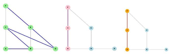
A graph, its coordinates, and the costs of moving from one node to another must be defined before we can fairly implement the BFS, DFS, and A* pathfinding algorithms. Let’s look at a network with six nodes, as seen in Figure 1, where A and F are the starting and the goal nodes, respectively.

Then the adjacency list of this diagram in Lisp may be expressed as:

;; Graph as adjacency list
(defparameter *example-graph*

‘((A B C)
(B A D E)
(C A F)
(D B)
(E B F)
(F C E)))

It is now necessary to have a function with ‘assoc’ to determine a node’s nearby neighbours, as indicated by the code below:

(defun neighbors (node graph)

(cdr (assoc node graph)))

Now we can define the BFS Lisp script for the aforementioned algorithms:

(in-package: pathfinding)

;;; BFS

(defun bfs (start goal graph)

(let ((queue (list (list start)))

(visited ‘()))

(loop while queue do

(let* ((path (pop queue))

(node (car (last path))))

(unless (member node visited)

(if (equal node goal)

(return path)

(progn

(push node visited)

(dolist (n (neighbors node graph))

(push (append path (list n)) queue)))))))))

The Lisp function for the DFS algorithms can also be written as:

(in-package :pathfinding)

;;; DFS

(defun dfs (start goal graph &optional (path ‘()) (visited ‘()))

(setq path (append path (list start)))

(cond

((equal start goal) path)

((member start visited) nil)

(t

(dolist (n (neighbors start graph))

(let ((result (dfs n goal graph path (cons start visited))))

(when result (return result)))))))

For the implementation of A* algorithms, we need one more piece of information about a connected graph: the coordinates of each node or the cost of each edge. In this discussion, we shall consider the coordinates only to measure the Euclidean distances between the nodes to select the shortest path from the origin to the goal.

In two dimensions, if the coordinates of the six nodes [A, B, C, D, E, F] are [(0,0), (1,0), (0,1), (2,0), (1,1), (0,2)], respectively, then the positions of the nodes can be expressed as:

(defparameter *example-positions*

‘((A (0 0)) (B (1 0)) (C (0 1))

(D (2 0)) (E (1 1)) (F (0 2))))

To measure the Euclidean distance between the nodes, a function ‘euclidean’ can be written as:

(in-package: pathfinding)



(defun euclidean (a b positions)

“Compute Euclidean distance between nodes A and B using POSITIONS alist.”

(let ((pa (cadr (assoc a positions)))

(pb (cadr (assoc b positions))))

(sqrt (+ (expt (- (first pa) (first pb)) 2)

(expt (- (second pa) (second pb)) 2)))))

With these two pieces of code, we can go for the implementation of the heuristic algorithm A*. The code is a bit complex, but a close observation can reveal its intricacy. Here’s the A* Lisp script:

(defun a-star (start goal graph &optional (positions *positions*))

“A* pathfinding from START to GOAL in GRAPH using Euclidean distance.”

(let ((open (list (list start)))

(visited ‘()))

(loop while open do

(setf open (sort open #’<

:key (lambda (path)

(+ (length path)

(euclidean (car (last path)) goal positions)))))

(let* ((path (pop open))

(node (car (last path))))

(unless (member node visited)

(if (equal node goal)

(return path)

(progn

(push node visited)

(dolist (n (neighbors node graph))

(unless (member n path)

(push (append path (list n)) open))))))))))

Implementation

The SBCL Common-Lisp platform is used to execute these codes. As SBCL is a free, open source program, it is downloadable and can be installed on a Windows-based PC. It is better to have a project directory ‘pathfinding’ for this implementation, as mentioned below, with six individual Lisp files.

pathfinding/

── package.lisp ; package declaration
── graph.lisp ; defines *graph* position and neighbors
── bfs.lisp ; define Breadth-First Search
── dfs.lisp ;define Depth-First Search
── astar.lisp ; define A* search
── run.lisp ; loads everything and runs

The project.lisp defines a project under which all the defined Lisp codes are integrated and can be executed using the run.lisp. The run.lisp loads all the necessary files for the execution. Since the project name is pathfinding, all the loaded Lisp files should have (in-package: pathfinding) at the top of the file. The package file is:

;; package.lisp

defpackage :pathfinding

(:use :cl)

(:export :bfs :dfs :a-star :example-graph :example-positions))

(in-package :pathfinding)

The run file is:

;; run.lisp

(load “package.lisp”)

(load “graph.lisp”) ; load *graph*. Position and neighbour helpers

(load “bfs.lisp”) ; load bfs.lisp

(load “dfs.lisp”) ;load dfs.lisp

(load “astar.lisp”) ;load astar.lisp

(in-package :pathfinding)

(format t “BFS path: ~a~%” (bfs ‘A ‘F *example-graph*))

(format t “DFS path: ~a~%” (dfs ‘A ‘F *example-graph*))

(format t “A* Path: ~a~%” (a-star ‘A ‘F *example-graph*)))

The search path from the start node A to the goal node F can be achieved by executing the run.lisp file with sbcl –load run.lisp

Execution

Command line execution of sbcl –load run.lisp will produce a result as shown in Figure 2.

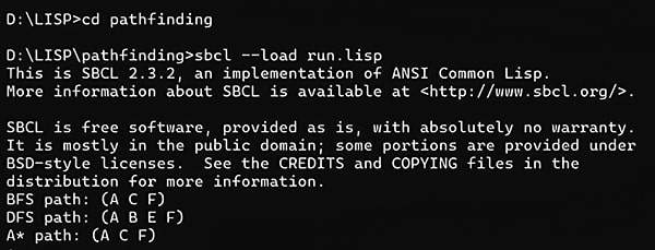
Paths of BFS, DFS, and A* to reach the goal F from the start node A are as follows:

BFS path: (A C F)

DFS path: (A B E F)

A* path: (A C F)

Visualisation

Here is how these three search strategies reach the goal node ‘F’. As can be seen from the graphs in Figure 2, BFS is an exhaustive search, while DFS and the A* search (with Euclidean distance) routes are identical with our six-node linked network. Colour codes are used to indicate search paths: orange for A* searches, pink for DFS searches, and green for BFS searches.

You can try and experiment with various heuristic distance metrics and graphs.