


In the previous articles in this series on SageMath, we explored graph theory extensively and recognised its significance in developing AI-based applications. In this sixth article in the series, we will revisit graph theory concepts due to their growing importance and conclude our discussion on graphs by looking at planar graphs.
Let us continue our discussion of directed graphs by exploring directed cycles. A directed cycle in a directed graph is a closed loop of directed edges. Let us determine whether the graph named Dgraph_12, generated by the SageMath code ‘dgraph12.sagews’ discussed in the previous article (OSFY, September 2024), contains a directed cycle. To do this, add the following line of code at the end of the ‘dgraph12.sagews’ program.
DG.is_directed_acyclic( )
We use CoCalc to execute SageMath code as before. Upon executing the modified program using CoCalc, we get the output ‘False’. Thus, it is clear that Dgraph_12 is cyclic. For example, 2–3–1–2 is a directed cycle of length 3 (see Figure 1 in the previous article).
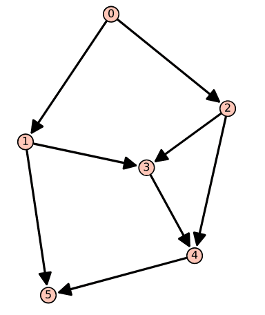
The discussion of directed cycles naturally leads us to another important type of directed graph: the directed acyclic graph (DAG). DAGs play a pivotal role in AI due to their ability to represent structures where information flows in a single direction without forming loops. This property is essential for modelling causal relationships and dependencies, making DAGs ideal for applications such as Bayesian networks and various machine learning algorithms. The acyclic nature of DAGs ensures that computations can be carried out efficiently without the risk of infinite loops, making them foundational in AI system design. The program ‘dacyclic16.sagews’ shown below generates a directed acyclic graph called Dag_16. Kindly note that programs and graphs discussed in this series are given continuous numbering for ease of reference. The following is the sixteenth complete SageMath program we have discussed in this series.
DAG = DiGraph( )
DAG.add_vertices([0, 1, 2, 3, 4, 5])
edges = [(0, 1), (0, 2), (1, 3), (1, 5), (2, 3), (2, 4), (3, 4), (4, 5)]
DAG.add_edges(edges)
DAG.show( )
The code does not require any explanation, as it is similar to the directed graphs we generated in the previous article of this series. The key difference is that there are no directed cycles in this graph. Upon executing the program ‘dacyclic16.sagews’ using CoCalc, we obtain the directed acyclic graph Dag_16, shown in Figure 1. From Figure 1, it is clear that Dag_16 contains no directed cycles. You can verify this by appending the line of code ‘DAG.is_directed_acyclic( )’ at the end of the program ‘dacyclic16.sagews’ and re-executing it. Upon execution of the modified program, you will get the output ‘True’, confirming that Dag_16 is indeed acyclic.
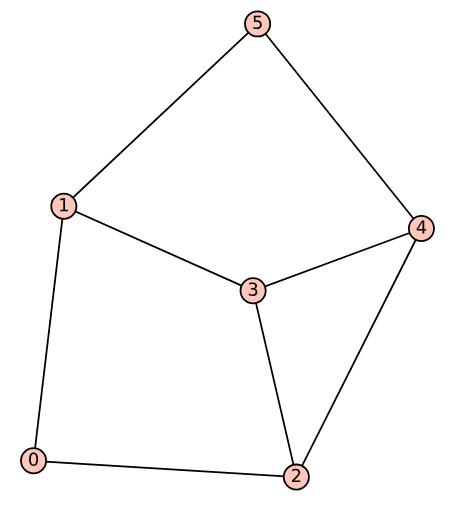
An important task often performed in graph theory is obtaining the corresponding undirected graph from a directed graph. To do this, add the following lines of code at the end of the ‘dacyclic16.sagews’ program.
UG = DAG.to_undirected( )
UG.show( )
Upon executing the modified program, the undirected graph corresponding to Dag_16, shown in Figure 2, is obtained.
Now, let us discuss weighted graphs (undirected), which we explored in the second article in this series (OSFY, February 2024). Operations research (OR) is the application of mathematical and analytical methods to optimise decisions and solve complex problems. For example, when dealing with distances in a graph, OR techniques can be used to find the shortest path between two vertices. Therefore, manipulating weighted graphs is an essential skill that every competent SageMath programmer should acquire. The program ‘wgraph17.sagews’, shown below, generates a weighted graph called Wgraph_17 and attempts to print the length of the shortest path between vertices 0 and 1 (line numbers have been included for clarity in the explanation).
1. G = Graph({0: {2: 11}, 1: {2: 77}, 2: {3: 22},
3: {0: 88, 1: 33}})
2. G.show(edge_labels=True)
3. shortest_path = G.shortest_path(0, 1)
4. shortest_path_len = G.shortest_path_length(0, 1)
5. print(shortest_path, ‘\n’, shortest_path_len)
Now, let us go through the code line by line to understand how it works. Line 1 creates a weighted directed graph G. The graph is defined by specifying edges and their weights using a dictionary. For example, the code fragment ‘0: {2: 11}’ means there is an edge from vertex 0 to vertex 2 with a weight of 11. Line 2 displays the graph with edge labels showing their weights. Line 3 computes the shortest path from vertex 0 to vertex 1 in the graph. The result is a list of vertices representing the path with the minimum total weight. Line 4 calculates the total length of the shortest path from vertex 0 to vertex 1. Finally, Line 5 prints the shortest path and its length.
Upon executing the program ‘wgraph17.sagews’ using CoCalc, we obtain the weighted graph Wgraph_17. The resulting graph, along with the (supposedly) shortest path and its length from vertex 0 to vertex 1, is shown in Figure 3.
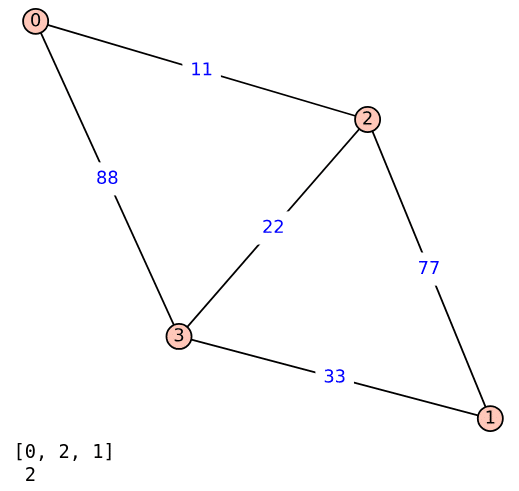
But there is something wrong with the output, right? The shortest path from 0 to 1 is shown as passing through vertex 2, and the distance is shown to be just 2. This suggests that while calculating the shortest path and its length, the code in lines 3 and 4 ignores the edge weights, leading to an incorrect result. Upon closer inspection of the graph Wgraph_17, it can be seen that the shortest path from 0 to 1 is actually 0–2–3–1, and the length of this path is 66. Now, we need to find the shortest path considering the edge weights. To do that, replace lines 3 to 5 of the program ‘wgraph17.sagews’ with the following three lines of code (line numbers have been included for clarity in the explanation).
3. shortest_path = G.shortest_paths(0, by_weight=True, algorithm=”Dijkstra_Boost”)
4. shortest_path_len = G.shortest_path_lengths(0, by_weight=True, algorithm=”Dijkstra_Boost”)
5. print(shortest_path, ‘\n’, shortest_path_len, ‘\n’, shortest_path_len[1])
Now, let us go through the code line by line to understand how it works. Line 3 calculates the shortest paths from vertex 0 to all other vertices in the graph G. The first parameter (0 in this case) specifies the source vertex from which the paths are calculated. The parameter ‘by_weight=True’ ensures that the shortest paths are determined based on the sum of the edge weights (i.e., the actual distance or cost) rather than just the number of edges. The parameter ‘algorithm=‟Dijkstra_Boost”’ specifies that Dijkstra’s algorithm should be used to compute the shortest paths (more on Dijkstra’s algorithm soon). The result, stored in shortest_path, is a dictionary where each key is a vertex, and the corresponding value is a list representing the shortest path from vertex 0 to that vertex.
Line 4 calculates the shortest path lengths (i.e., the total weight or distance) from vertex 0 to all other vertices in the graph G. The parameters and their meanings are the same as those used in Line 3. The result, stored in shortest_path_len, is a dictionary where each key is a vertex, and the corresponding value is the total weight (length) of the shortest path from vertex 0 to that vertex.
Line 5 prints the results of the shortest path calculations. It prints the dictionary containing the shortest paths from vertex 0 to all other vertices, the dictionary containing the shortest path lengths (distances) from vertex 0 to all other vertices, and the shortest path length (distance) specifically from vertex 0 to vertex 1.
Upon executing the modified program, the following additional output will be displayed on the screen along with Wgraph_17.
{0: [0], 1: [0, 2, 3, 1], 2: [0, 2], 3: [0, 2, 3]}
{0: 0, 1: 66, 2: 11, 3: 33}
66
Now, let us analyse this output. The first line shows the shortest_path dictionary ({0: [0], 1: [0, 2, 3, 1], 2: [0, 2], 3: [0, 2, 3]}), which details the shortest path from vertex 0 to each of the other vertices. For example, for vertex 0, the path is [0], meaning the shortest path from 0 to itself is trivially just 0. For vertex 1, the path is [0, 2, 3, 1], indicating that the shortest path from 0 to 1 passes through vertices 2 and 3. The second line shows the shortest_path_len dictionary ({0: 0, 1: 66, 2: 11, 3: 33}), which represents the corresponding shortest path lengths (i.e., the total weight of the paths) from vertex 0 to each of the other vertices. For example, the distance from vertex 0 to itself is 0, as expected, since no travel is involved. The distance to vertex 1 is 66, which corresponds to the sum of the edge weights along the path [0, 2, 3, 1]. This is calculated as 11 (from 0 to 2) + 22 (from 2 to 3) + 33 (from 3 to 1) = 66. Finally, the third line shows the specific shortest path length from vertex 0 to vertex 1, which, as mentioned earlier, is 66.
Now, a word about Dijkstra’s algorithm, developed by one of the greatest computer scientists of all time, Edsger W. Dijkstra (pronounced ‘Dykstra’). In his honour, the most influential paper in distributed computing is awarded the annual Dijkstra Prize. Dijkstra developed this algorithm in 1956 to find the shortest path in a graph when all edge weights are positive (and yes, edge weights can also be negative). The algorithm identifies the shortest path from a given source vertex to every other vertex in the graph. A variant of Dijkstra’s algorithm, known as uniform cost search, is widely used in artificial intelligence.
In the modified ‘wgraph17.sagews’ program discussed earlier, the parameter algorithm in lines 3 and 4 offers several options beyond Dijkstra_Boost, including BFS, Dijkstra_NetworkX, and Bellman-Ford_Boost. It is important to note that Dijkstra_Boost (the Boost Graph Library implementation in C++) and Dijkstra_NetworkX (the NetworkX implementation in Python) are two different implementations of Dijkstra’s algorithm. But how do the other algorithms differ from Dijkstra’s? They vary based on the types of graphs they can handle, their execution speed, and other factors. For example, the Bellman-Ford algorithm can handle graphs with negative edge weights, as long as there is no cycle with negative weight. The study of distances in graphs is a significant field in computer science with countless applications. Although a detailed discussion is beyond the scope of this series, I strongly encourage you to explore this area further on your own.
Next, we will dive into searching in graphs. Whether an AI-based application is navigating a maze, playing chess, or deciding what to do next in a conversation, it is all about searching for the best option among countless possibilities. In AI, graph search is key to finding optimal or most efficient solutions. For instance, in path-finding algorithms like Dijkstra’s or A*, searching helps determine the shortest or least costly route from one point to another, which is vital in robotics, autonomous vehicles, and game development. In decision-making systems, searching through a graph of possible moves or actions allows AI to assess potential outcomes and select the best course of action, a process that is fundamental in areas like machine learning, planning, and strategy games.
In this discussion, we will focus on two classical graph searching algorithms, also known as graph traversal algorithms: Breadth-First Search (BFS) and Depth-First Search (DFS). BFS explores a graph level by level, starting from a given vertex, called the root. It visits all neighbouring vertices at the current depth before moving on to those at the next depth level. Imagine you are at the entrance of a maze and want to explore it systematically. First, you check all the rooms (vertices) directly connected to the entrance. Then, you move to the rooms connected to those, continuing this process layer by layer.
On the other hand, DFS dives deep into the graph, exploring as far as possible along one path before backtracking. Think of DFS as selecting a corridor in the maze and following it until you reach a dead end. At that point, you backtrack to the last branching point and choose a different corridor to explore.
While BFS requires more memory to process since it keeps track of all the vertices at the current level, it guarantees finding the shortest path to the destination. DFS, in contrast, uses less memory because it only needs to store the current path, but it may not always find the shortest path to the destination.
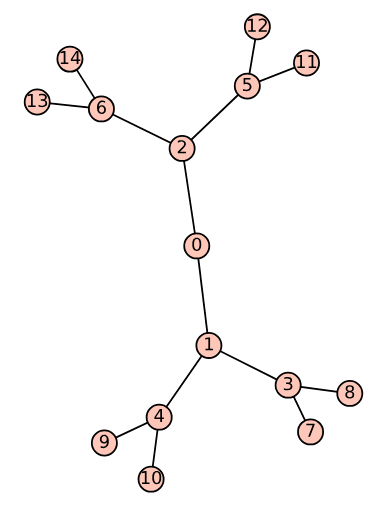
For ease of understanding, we will first perform BFS and DFS on a tree. The program ‘tree18.sagews’ shown below generates a tree called Tree_18.
T = Graph({0: [1, 2], 1: [3, 4], 2: [5, 6], 3: [7, 8], 4: [9, 10], 5: [11, 12], 6: [13, 14]})

T.show( )
Notice that the first line of the above program is similar to the first line of the SageMath program ‘wgraph17.sagews’, so no explanation is needed. Upon executing the program ‘tree18.sagews’ using CoCalc, we obtain the tree Tree_18, as shown in Figure 4.
Now, let us perform BFS on the tree Tree_18. To do this, add the following lines of code at the end of the ‘tree18.sagews’ program. The BFS will begin from vertex 0.
bfs_order = list(T.breadth_first_search(0))
print(“BFS Order:”, bfs_order)
Upon executing the modified program, the following additional output will be displayed on the screen.
BFS Order: [0, 1, 2, 3, 4, 5, 6, 7, 8, 9, 10, 11, 12, 13, 14]
Now, let us perform DFS on the tree Tree_18. To do this, add the following lines of code at the end of the ‘tree18.sagews’ program. The DFS will begin from vertex 0.
dfs_order = list(T.depth_first_search(0))
print(“DFS Order:”, dfs_order)
Upon executing the modified program, the following additional output will be displayed on the screen.
DFS Order: [0, 2, 6, 14, 13, 5, 12, 11, 1, 4, 10, 9, 3, 8, 7]
A comparison of the BFS and DFS traversal orders for the given tree highlights the fundamental differences in how these algorithms explore a graph. BFS explores all the neighbours at the current depth level before moving on to nodes at the next level, resulting in a level-by-level traversal of the tree that starts from the root (vertex 0) and expands outward. In contrast, DFS explores as far as possible along each branch before backtracking, leading to a traversal that delves deep into one branch (for example, 0 – 2 – 6 – 14) before returning to explore other branches. These differences make BFS more suitable for finding the shortest path in unweighted graphs, while DFS is often employed for tasks like exploring all possible configurations or detecting cycles in graphs.
Now, let us perform BFS and DFS on a cycle to better understand the differences between the two algorithms. The program ‘cycle19.sagews’ shown below generates a cycle called Cycle_19.
C = graphs.CycleGraph(15)

C.show( )
Upon executing the program ‘cycle19.sagews’ using CoCalc, we obtain the cycle Cycle_19, as shown in Figure 5.
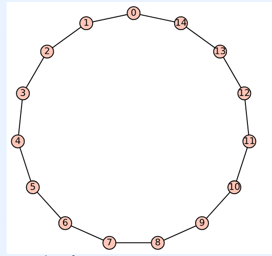
Now, let us perform BFS on the cycle Cycle_19. To do this, add the following lines of code at the end of the ‘cycle19.sagews’ program. The BFS will begin from vertex 14.
bfs_order = list(C.breadth_first_search(14))
print(“BFS Order:”, bfs_order)
Upon executing the modified program, the following additional output will be displayed on the screen.
BFS Order: [14, 0, 13, 1, 12, 2, 11, 3, 10, 4, 9, 5, 8, 6, 7]
Now, let us perform DFS on the cycle Cycle_19. To do this, add the following lines of code at the end of the ‘cycle19.sagews’ program. The DFS will begin from vertex 14.
dfs_order = list(C.depth_first_search(14))
print(“DFS Order:”, dfs_order)
Upon executing the modified program, the following additional output will be displayed on the screen.
DFS Order: [14, 13, 12, 11, 10, 9, 8, 7, 6, 5, 4, 3, 2, 1, 0]
Now, let us compare the BFS and DFS traversal sequences. BFS begins at the initial vertex (14 in this case) and explores all its immediate neighbours before progressing to the neighbours of those vertices. This approach leads to a traversal pattern that alternates between moving left and right along the cycle, covering the vertices in a more evenly distributed manner. On the other hand, DFS also starts at vertex 14 but dives as deeply as possible along one path before backtracking. In this scenario, it traverses the entire cycle in a single direction, visiting each vertex in sequence until it reaches the last vertex (0 in this case).
Before we conclude our discussion of graphs in this SageMath series, we need to cover one more important type of graph: planar graphs. A planar graph is a graph that can be drawn on a flat surface, like a piece of paper, in such a way that its edges do not cross each other. In other words, you can arrange the vertices (points) and edges (lines connecting the points) of the graph so that no two edges intersect except at their endpoints (vertices). If it is impossible to draw a graph without edges crossing, then that graph is non-planar. For example, a triangle is a planar graph because you can easily draw it without any edges crossing. Now, let us check whether Cycle_19 is planar or not. To do this, add the following line of code at the end of the program ‘cycle19.sagews’.
C.is_planar( )
Upon executing the modified program, the message ‘True’ is displayed, verifying that Cycle_19 is indeed planar, as can be easily confirmed from Figure 5. Please also verify that Wgraph_17 and Tree_18 are planar graphs.
Now, let us explore an important aspect of planar graphs: a planar graph can be drawn in a non-planar way. This means that even though the graph can be represented without any crossing edges, it might still be drawn in a way that causes some edges to intersect. Take, for example, the complete graph K4, which consists of four vertices, with every pair of vertices connected by an edge. K4 is a planar graph because it can be drawn without any edges crossing. The code below displays the complete graph K4 and also checks whether it is planar.
K4 = graphs.CompleteGraph(4)
K4.show( )
K4.is_planar( )
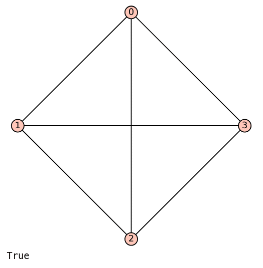
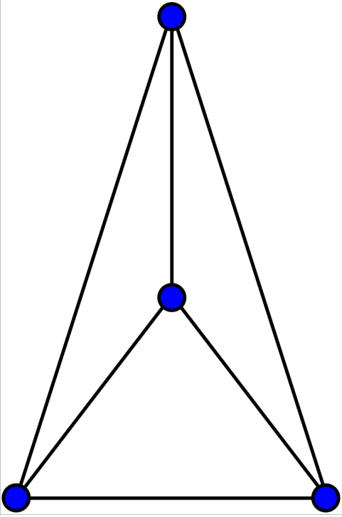
Upon executing the code above, a non-planar drawing of K4 is displayed, as shown in Figure 6. However, since the message ‘True’ appears, it indicates that K4 can indeed be drawn as a planar graph. Figure 7 shows a planar drawing of K4 (courtesy of Wikipedia). I encourage you to read the Wikipedia article on ‘Planar Graph’ to learn more about this topic.
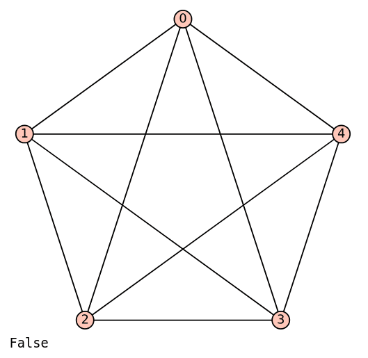
Now, let us examine a straightforward example of a non-planar graph: the complete graph K5. The code below displays the complete graph K5 and checks whether it is planar.
K5 = graphs.CompleteGraph(5)
K5.show( )
K5.is_planar( )
Upon executing the code above, a (non-planar) drawing of K5 is displayed, as shown in Figure 8. Please take some time to verify that it is impossible to draw K5 without edges crossing, which confirms that it is non-planar.
Now, it is time to wrap up our discussion. We have been exploring graph theory for a while now, and while we could continue delving into it and still only scratch the surface, what we have covered should provide you with a strong foundation to begin your journey into graph theory and its applications in computer science and AI. Although we will occasionally revisit graph theory, our focus will shift to cybersecurity, another hot topic in computer science, starting with the next article. In the upcoming articles, we will explore how various concepts in cybersecurity can be implemented and tested using SageMath.


