Follow this guide to leverage your enterprise data with a self-hosted AI assistant, powered by the semantic search capabilities of open source vector databases.

In today’s fast-paced enterprise environment, the volume of internal documentation—from support tickets and confluence pages to technical specifications and project wikis—grows exponentially. For knowledge workers, this deluge of information presents a significant challenge. Traditional, keyword-based search engines are often too rigid and brittle to navigate this unstructured sea of data. A search for ‘server performance issue’ may fail to find a document titled ‘optimising backend latency’, despite the two topics being semantically identical. The inability to quickly access relevant, up-to-date information represents a critical bottleneck for productivity and innovation.

This challenge has a modern, robust solution: retrieval-augmented generation (RAG). RAG is an AI framework that fundamentally shifts how large language models (LLMs) operate. Instead of relying solely on their pre-trained knowledge, which can be outdated or contain inaccuracies, RAG systems first retrieve information from a specified external knowledge base before generating a response. This approach provides a ‘factual grounding’ for the LLM, effectively mitigating the notorious problem of AI ‘hallucinations’. The resulting answers are not only more accurate but can also be directly linked to their source documents, a feature that significantly enhances user trust and transparency.

At the heart of this architecture lies the vector database, an indispensable component that serves as the external knowledge base. Unlike traditional databases, which are optimised for the structured world of rows and columns, a vector database is engineered for the high-dimensional, unstructured data of text, images, and audio. Its core function is to store, manage, and query data in the form of vectors, which are numerical representations of an object’s features. This design enables lightning-fast ‘semantic search’ based on the meaning and context of the data, a capability that traditional databases simply cannot match.

For open source administrators and developers, the RAG paradigm presents a particularly compelling opportunity. Historically, making a large language model proficient in an organisation’s proprietary data required an expensive and computationally intensive process known as fine-tuning. This meant retraining a massive model for every new dataset or domain-specific requirement. RAG, by contrast, offers a far more cost-effective and flexible alternative. By connecting an LLM to an organisation’s knowledge base via a vector database, developers can rapidly create intelligent applications without the prohibitive financial and computational overhead of model retraining. This makes generative AI technology more broadly accessible and usable, positioning open source solutions as the ideal choice for those who value flexibility, control, and a lower total cost of ownership.

The foundation: Selecting your FOSS vector database

Building a production-ready RAG system requires a robust and scalable vector database. These systems are designed to manage vast volumes of unstructured data by storing and indexing high-dimensional vector embeddings. The true power of these databases for enterprise applications lies in their ability to perform semantic searches, which retrieve information based on conceptual similarity rather than just keyword matches. Beyond basic search, enterprise-class vector databases offer crucial features such as metadata filtering and scalability to handle growing datasets without compromising performance.

While commercial solutions like Pinecone, Weaviate, and Chroma offer managed services, a vibrant ecosystem of open source alternatives provides compelling self-hosted options. This ecosystem is not a monolith; each solution possesses a distinct architectural philosophy and a unique set of strengths, making the choice a strategic decision based on the specific needs of a project.

Weaviate

As a cloud-native, open source vector database, Weaviate is designed to store both objects and vectors, seamlessly combining vector search with structured filtering. Its architecture is built in Go for speed and reliability, and it offers native support for horizontal scaling, making it a strong choice for mission-critical applications. Its ease of deployment via Docker and Kubernetes and its robust Python client make it highly accessible for developers prototyping locally or deploying at scale.

Qdrant

Known for its high performance, Qdrant leads in requests-per-second and low latency, with response times as low as milliseconds for millions of vectors. Its performance-first design makes it an ideal choice for applications where speed is paramount, such as real-time recommendation engines or high-traffic search APIs. Qdrant also offers built-in features like vector compression and multi-vector support, which can significantly reduce memory usage and enhance search experiences.

Milvus

Built for large-scale distributed systems, Milvus is a high-performance vector database that excels at managing massive datasets for generative AI applications. Its architecture is designed to handle immense data scales, making it a go-to solution for companies with petabytes of unstructured data. For local development and smaller projects, the Milvus Lite option provides a convenient, file-based solution that doesn’t require a full server setup, catering directly to the needs of individual developers and small teams. Milvus’s strong integration with Docker makes it easy for Linux administrators to get started.

The pgvector extension

For organisations already invested in the PostgreSQL ecosystem, pgvector offers a simple and powerful alternative. Instead of deploying and managing a separate database system, pgvector allows for the storage and retrieval of vector embeddings directly within a PostgreSQL instance. This option appeals to administrators who value integrated, battle-tested tooling and a single-database approach for their applications.

Table 1 provides a comparison to help guide the decision-making process based on specific project requirements.

Database	Primary strength	Deployment	Supported features	Community/framework support
Weaviate	Cloud-native, scalability	Docker, Kubernetes, Cloud	Hybrid search, RAG, Metadata filtering	LangChain, LlamaIndex, Go, Python, Java
Qdrant	High performance, speed	Docker, Cloud	Hybrid search, Multi-vector, Quantization	LangChain, LlamaIndex, Python, Rust, Go
Milvus	Scalability, large datasets	Docker, Kubernetes, Cloud	Hybrid search, Multi-vector, Replication	LangChain, LlamaIndex, Python, Java, Go
pgvector	Integration, simplicity	PostgreSQL Extension	L distance, Inner product, Cosine similarity	LangChain, LlamaIndex, Python, Go, Rust

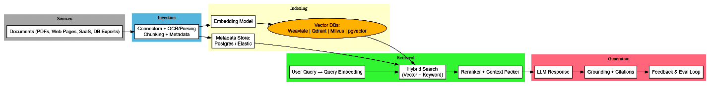
The blueprint: The RAG system architecture

An enterprise RAG system is more than just a vector database; it is a meticulously engineered pipeline that orchestrates the flow of data from raw documents to a contextualized AI response. The process can be broken down into a series of core stages, each critical to the system’s overall performance and accuracy. The success of this pipeline is acutely dependent on the quality of data preparation and ingestion, a foundational step that is often underestimated. A technically advanced vector database cannot compensate for a flawed ingestion process.

Ingestion and chunking

The first step involves preparing the source data. Unstructured documents, such as PDFs or web pages, must be broken down into smaller, logical pieces, or ‘chunks’, for the LLM to process. This process is crucial because a chunk that is too large can contain irrelevant information, while a chunk that is too small can lose essential context. The effectiveness of the entire RAG system is directly tied to the quality of this step, as poor chunking leads to irrelevant retrieval and, consequently, a poor final response.

Embedding generation

Once the documents are chunked, each text chunk is passed through an embedding model. This model converts the text into a dense numerical array called a ‘vector embedding’. These embeddings are designed to encode the semantic meaning of the text, such that chunks with similar meaning or context will have vectors that are mathematically ‘close’ to one another in a high-dimensional space.

Vector storage and indexing

The newly generated vector embeddings, along with their associated metadata, are then stored and indexed in the chosen vector database. This indexing process is what enables the database to perform a lightning-fast approximate nearest neighbour (ANN) search, quickly finding the most relevant vectors from a massive dataset.

Retrieval

This is the ‘R’ in RAG. When a user submits a query, it undergoes the same embedding process. The resulting query vector is then used to perform a similarity search in the vector database. The system retrieves the top ‘k’ most relevant chunks—those whose vectors are mathematically closest to the query vector—and pulls them from the database.

Augmented generation

The ‘G’ in RAG. The final stage involves passing the user’s original query and the newly retrieved, relevant document chunks together to the large language model. The LLM uses this ‘augmented context’ to generate a response that is not only coherent and well-written but also factually grounded in the provided source material.

Practical guide: Building an RAG system on Linux

For the open source enthusiast, a fully self-hosted, Linux-native RAG system is not a distant vision but a practical reality. This guide provides a hands-on blueprint using Qdrant and a Python-based orchestration framework to create a functional prototype. This will be the first part in the overall series. In the coming parts, I will try to cover the rest of the solutions mentioned in the above section.

To build a RAG system that acts as a knowledgeable AI assistant for your enterprise documents, we will walk through a complete, self-hosted implementation using Python, an open source vector database like Qdrant, and a FOSS embedding model.

Before stepping into the journey of implementation, let us quickly comprehend the basics of the product. This should help you understand each step better and configure accordingly.

Term	Meaning
Collections	Collections define a named set of points that you can use for your search.
Payload	A payload describes information that you can store with vectors.
Points	Points are a record which consists of a vector and an optional payload.
Search	Search describes similarity search, which sets up related objects close to each other in vector space.
Explore	Explore includes several APIs for exploring data in your collections.
Hybrid queries	Hybrid queries combine multiple queries or perform them in more than one stage.
Filtering	Filtering defines various database-style clauses, conditions, and more.
Optimizer	Optimizers are options to rebuild database structures for faster search. These include a vacuum, a merge, and an indexing optimizer.
Storage	Storage is the configuration of storage in segments, which include indexes and an ID mapper.
Indexing	Indexing lists and describes available indexes. These include payload, vector, sparse vector, and a filterable index.
Snapshots	Snapshots describe the backup/restore process (and more) for each node at specific times.

 

Step 1: Setting up the environment

Before you begin, you need to ensure your Linux system has the necessary tools. This includes Python .8+ and Docker. You will also need to install the required Python libraries.

First download the latest Qdrant image from the Docker Hub:

docker pull qdrant/qdrant

Then run the service:

docker run -p 6333:6333 -p 6334:6334 \

-v “$(pwd) /qdrant_storage: /qdrant/storage:z” \

qdrant/qdrant

Under the default configuration all data will be stored in the
./qdrant_storage directory. This will also be the only directory that both the container and the host machine can see.

Qdrant is now accessible:

• REST API: localhost:6333
• Web UI: localhost:6333/dashboard
• GRPC API: localhost:6334

Step 2: Initialising Qdrant client, creating a collection, and generating embeddings

Now that Qdrant is running and your Python environment is set up, let’s start writing some code to interact with it. We’ll initialise the Qdrant client, create a collection to store our vectors, and use a pre-trained model to generate vector embeddings from text.

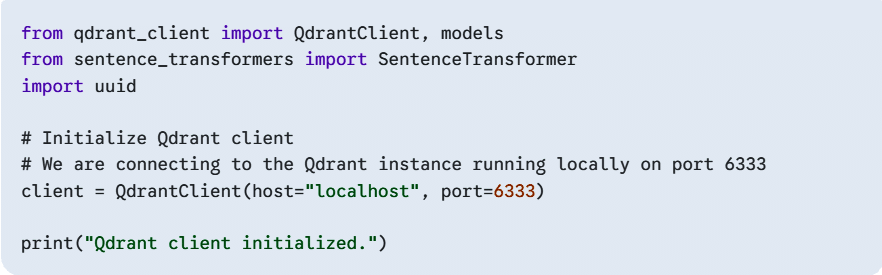
Initialise the Qdrant client

First, open a new Python file (e.g., qdrant_tutorial.py) in your project directory and add the codes below. We need to connect to our running Qdrant instance.

from qdrant_client import QdrantClient, models

from sentence_transformers import SentenceTransformer

import uuid

# Initialize Qdrant client

# We are connecting to the Qdrant instance running locally on port 6333

client = QdrantClient (host=”localhost”, port=6333)

print(“Qdrant client initialized.”)

The QdrantClient is the main interface for interacting with your Qdrant database. We’re connecting to localhost on port 6333, which is the default gRPC port for Qdrant in Docker.

Define our data and embedding model

To demonstrate semantic search, we need some text data and a way to convert that text into numerical vectors (embeddings). We’ll use the SentenceTransformer library, which provides easy access to pre-trained models.

# Our sample data

documents = [

“Qdrant is a vector similarity search engine.”,

“It helps in finding relevant information quickly.”,

“Vector databases are essential for modern AI applications like RAG.”,

“Machine learning models can generate powerful embeddings.”,

“The Qdrant dashboard provides a great overview of collections.”,

“SentenceTransformers can create semantic vector embeddings.”,

“Langchain often integrates with Qdrant for RAG applications.”,

“Understanding embeddings is key to effective vector search.”

]

# Initialize a SentenceTransformer model for generating embeddings

# ‘all-MiniLM-L6-v2’ is a good balance of performance and size

embedding_model = SentenceTransformer(“all-MiniLM-L6-v2”)

print(“Embedding model loaded.”)

Here, documents is a list of simple text strings that we’ll convert into vectors. The SentenceTransformer(“all-MiniLM-L6-v2”) loads a pre-trained model capable of generating high-quality semantic embeddings. This model will convert each sentence into a fixed-size numerical vector where semantically similar sentences will have vectors that are numerically close to each other.

Create a Qdrant collection

Before we can add vectors, we need to create a ‘collection’ in Qdrant. A collection is like a table in a relational database, but it’s designed specifically for storing vectors and their associated metadata. When creating a collection, you must specify the vector_size (the dimensionality of your embeddings) and the distance metric (how similarity between vectors is calculated).

collection_name = “my_first_collection”

# Get the vector size from our embedding model

# The ‘all-MiniLM-L6-v2’ model produces 384-dimensional vectors

vector_size = embedding_model.get_sentence_embedding_dimension()

# Check if the collection already exists and delete it if it does

# This is useful for re-running the tutorial script

if client.collection_exists(collection_name=collection_name):

client.delete_collection(collection_name=collection_name)

print(f”Collection ‘{collection_name}’ deleted (if it existed).”)

# Create the collection

client.create_collection(

collection_name=collection_name,

vectors_config=models.VectorParams(size=vector_size, distance=models.Distance

.COSINE),

)

print(f”Collection ‘{collection_name}’ created with vector size {vector_size} and

Cosine distance.”)

• collection_name: A unique name for our collection.
• vector_size: Obtained directly from embedding_model.get_sentence_embedding_dimension(). It’s crucial that this matches the output size of your embedding model.
• models.Distance.COSINE: Cosine similarity is a common and effective distance metric for text embeddings. It measures the cosine of the angle between two vectors, ranging from -1 (opposite) to 1 (identical).

The client.collection_exists and client.delete_collection lines are included for convenience, allowing you to run the script multiple times without errors if the collection already exists.

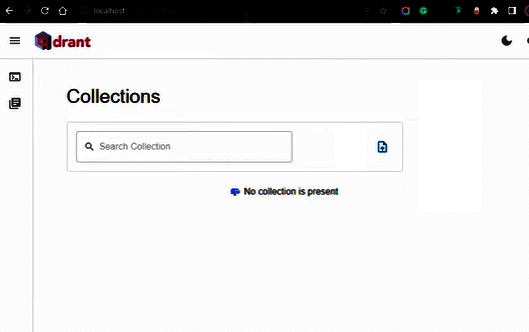
Figure 3 gives a visual representation of the concept of creating a collection, and presentation of collection_name and vector_size.

You should be able to see the newly created collection in your Qdrant user interface.

Generate embeddings and upsert into Qdrant

Now we’ll generate embeddings for each of our documents and then ‘upsert’ (insert or update) them into our Qdrant collection. Each point in Qdrant consists of a unique ID, the vector itself, and optionally a payload (metadata associated with the vector).

points = []

for i, doc in enumerate(documents):

vector = embedding_model.encode(doc).tolist() # Convert numpy

array to list

point_id = str(uuid.uuid4()) # Generate a unique ID for each point

payload = {“text”: doc, “index”: i} # Store the original text and

an index as metadata

points.append(

models.PointStruct(

id=point_id,

vector-vector,

payload=payload,

)

)

client.upsert(

collection_name=collection_name,

wait=True, # Wait for the operation to complete

points=points,

)

print(f”Upserted {len(points)} points into ‘{collection_name}’.”)

# Get collection info to verify the number of points

collection_info = client.get_collection(collection_name

=collection_name)

print (f”Current number of points in collection: {collection_info

.points_count}”)

• embedding_model.encode(doc).tolist(): This takes a document, generates its embedding as a NumPy array, and then converts it to a Python list, which Qdrant expects.
• uuid.uuid4(): Generates a universally unique identifier (UUID) for each point. This ensures that each vector has a distinct ID in Qdrant.
• payload: This is a dictionary where you can store any additional metadata you want to associate with your vector. Here, we’re storing the original text and its index. This metadata is extremely powerful for filtering and enriching search results.
• client.upsert(): This method sends our points to Qdrant. wait=True makes the client wait for the operation to complete before continuing.

This process essentially transforms your raw text data into a searchable, semantic database.

Step 3: Performing a semantic search

Now that your Qdrant collection is populated with vector embeddings, you can perform a semantic search. This is the core of the tutorial’s purpose, as it allows you to find relevant information based on the meaning of your query, rather than just matching keywords.

To perform a search, first convert your search query into a vector using the same SentenceTransformer model you used for your documents. Qdrant then finds and returns the points (documents) in the collection with the most similar vectors.

Encode the search query

You need to use the exact same model to encode your query as you used for the documents. This ensures that the query vector and document vectors exist in the same vector space, making them comparable.

# The query text. You can change this to anything you want to search for.

query_text = “I’m looking for a tool for creating vector embeddings.”

# Encode the query text into a vector

query_vector = model.encode (query_text).tolist()

Perform the search

The client.search() method is the main function for querying your Qdrant collection. You provide it with the collection name, the query vector, and a limit to specify the number of results you want.

# Perform the semantic search

search_results = client.search(

collection_name=collection_name,

query_vector-query_vector,

limit=3 # Retrieve the top 3 most similar results

)

print(“\nSearching for: ‘{query_text}’\n”)

print(“-” * 30)

The client.search() call sends your query vector to Qdrant. The database then efficiently finds the vectors that are closest to your query vector based on the distance metric you defined (Cosine distance in this case).

Display the results

The search results are a list of ScoredPoint objects, which contain the point’s ID, its vector, the payload, and most importantly, a score that indicates the similarity between the query and the result. A higher score means greater similarity.

# Display the results

for result in search_results:

text_payload= result.payload.get(‘text’, ‘No text found’)

score result.score

print (f”Score: {score:.4f} -> Text: ‘{text_payload}’”)

print(“-” * 30)

By accessing the payload of each result, you can retrieve the original text associated with the vector, making the results human-readable.

Beyond the basics: Scaling and optimisation

The system described above provides a solid foundation for a prototype, but an enterprise-grade RAG solution requires more sophisticated techniques to ensure high-quality, reliable results. A simplistic similarity search is often insufficient for production workloads. A high-quality RAG system must be optimised to ensure that the retrieved information is not just similar but also highly relevant.

One critical enhancement is hybrid search, which combines the power of semantic (vector) search with traditional keyword-based search. While semantic search excels at finding conceptual matches, keyword search is essential for retrieving specific names, dates, or product codes that may not be semantically similar but are critical for an accurate response. By performing both searches and intelligently combining the results, the system can significantly improve relevance and recall.

Another advanced technique is re-ranking. After the initial retrieval, a re-ranker can be used as a post-processing step to fine-tune the order of the search results. This process, though computationally more expensive, ensures that the most relevant chunks are presented to the LLM, leading to more precise and coherent generated text.

For enterprise-level deployments, scalability and security are paramount. Open source vector databases are built to handle these challenges. Solutions like Weaviate and Milvus offer native support for horizontal scaling and can be deployed on platforms like Kubernetes to manage growing data volumes and query loads. For data management, modern vector databases support dynamic updates and metadata filtering, allowing for continuous synchronisation of the knowledge base and more precise query capabilities. Security is also a key consideration, with some open source solutions offering enterprise-grade features such as role-based access control (RBAC) to restrict sensitive information retrieval based on authorisation levels.

Empowering your enterprise knowledge base

The tools and frameworks are now in place for open source administrators and developers to build powerful, self-hosted AI applications. The RAG framework provides a clear, cost-effective, and powerful path to make large language models a truly viable asset for enterprise knowledge management. By leveraging the flexibility and performance of open source vector databases like Qdrant, Weaviate, Milvus, or even the battle-tested pgvector extension, organisations can transform their internal data into an intelligent, accessible, and continuously up-to-date resource. The blueprint has been provided, and the power to innovate is in the hands of the community.