In the last column, we had discussed some basic algorithms and methodologies. Now we will generalise the scheme of an algorithm. It will have the following properties:
- Arranged in an ordered sequence that you can number (as steps)
- Unambiguous and well-defined
- Halts in finite time (i.e., the algorithm terminates!)
And we will generally stumble upon the following algorithmic operations:
- Sequential operations—where instruction sets are executed in order
- Conditional operations—that ask a true/false question and then select the next instruction based on the answer
- Iterative operations (loops)—that repeat the execution of a set of instructions
It should be emphasised that, as we discussed before, not every problem has a ‘good’ algorithmic solution. There are:
- Halting problems (unsolvable problems)—for which no algorithm exists to solve the problem.
- Travelling salesman problems (intractable problems)—algorithms that take too long to solve the problem.
- Problems with no known algorithmic solution.
Pseudo code structure
The algorithm may contain the following elements: IF-THEN-ELSE.
Binary choice on a given Boolean condition is indicated by: IF, THEN, ELSE, and ENDIF. The general representation is:
IF condition THEN
     sequence 1
ELSE
     sequence 2
ENDIF
Please note that the ELSE keyword and “sequence 2” are optional.
WHILE: The loop is executed only if the condition is true. The ‘WHILE construct’ is used to specify a loop with a test at the top. WHILE and ENDWHILE are to identify the beginning and ending of the loop. The general form for WHILE is:
WHILE condition
     sequence
ENDWHILE
CASE: In order to handle mutually exclusive conditions, we can go for CASE. CASE, OF, OTHERS, and ENDCASE are the keywords commonly used for this. The alternatives available will be represented with the help of ‘conditions’.
CASE expression OF
     condition 1 : sequence 1
     condition 2 : sequence 2
     ...
     condition n : sequence n
     OTHERS:
     default sequence
ENDCASE
REPEAT-UNTIL: This is quite akin to WHILE, but here the operation is performed at the bottom of the loop.
REPEAT
     sequence
UNTIL condition
FOR: We employ FOR and ENDFOR in our algorithm for iterating the code block for a specific number of times. It is also called the “counting” loop.
FOR iteration bounds
     sequence
ENDFOR
EXCEPTION HANDLING: The following code elucidates this.
BEGIN
     statements
EXCEPTION
     WHEN exception type
          statements to handle exception
     WHEN another exception type
          statements to handle exception
END
You can also utilise methods like NESTED CONSTRUCTS, INVOKING SUBPROCEDURES to construct elegant and powerful algorithms.
We can define seven golden rules for writing algorithms:
- Use good code and good English.
- Ignore unnecessary details
- Take advantage of programming shorthand
- Be context specific
- Don’t lose sight of the base model
- Always check for balance (can be easily implemented in a language)
Implementation
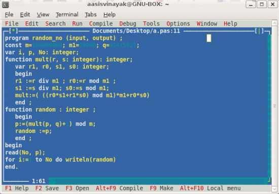
Let’s write the code that produces a random number. Random number generation is an important tool in simulation building and scientific computing. In order to elucidate the implementation of the algorithm, I have written the code in Pascal.
program random_no (input, output) ;
const m=100000000; m1=10000; q=31415821;
var i, p, No: integer;
function mult(r, s: integer): integer;
     var r1, r0, s1, s0: integer;
     begin
     r1 :=r div m1 ; r0:=r mod m1 ;
     s1 :=s div m1; s0:=s mod m1;
     mult:=( ((r0*s1+r1*s0) mod m1)*m1+r0*s0)
     end ;
function random : integer ;
     begin
     p:=(mult(p, q)+1) mod m;
     random :=p;
     end ;
begin
read(No, p);
for i:=1 to No do writeln(random)
end.
It’s assumed that you are skilled in grasping the meaning of simple codes. You can try this in your preferred Pascal compiler. (Figure 1 shows the code in Free Pascal Compiler, which I installed for trial.)

Euclid’s Algorithm: A response to the queries
Many readers who tried the algorithms in the reference books (suggested in the last column) posed the question concerning the simplification of Euclid’s algorithm and the base problem. As it was given as a problem, many of ‘our passengers’ got wedged between the lines!
For those who have not tried the exercises (if you don’t have the book, you can find many online resources), here is a prologue to the problem:
Let a and b be integers, with a ≥ b ≥ 0. Using the division with the remainder property, define the integers r0 , r1 , . . . , rλ+1 , and q1 , . . . , qλ , where λ ≥ 0, as follows:
          a = r0 ,
          b = r1,
     r0 = r1 q1 + r2     (0 < r2 < r1 ),
          .
          .
          .
ri−1 = ri qi + ri+1   (0 < ri+1 < ri ),
          .
          .
          .
rλ−2 = rλ−1 qλ−1 + rλ (0 < rλ < rλ−1 ),
rλ−1 = rλqλ          (rλ+1 = 0).
From the given definitions λ = 0 if b = 0, and λ > 0 for all other cases. Then we have rλ =√gcd(a, b). Moreover, if b > 0, then λ ≤ log b/ log ϕ + 1, where ϕ := (1 + 5)/2 ≈ 1.62.
Algorithm: If we could furnish input as a and b, where a and b are integers such that a ≥ b ≥ 0, we can compute d = gcd(a, b) as exemplified below:
r ← a, r ← b
while r = 0 do
     r ← r mod r
     (r, r ) ← (r , r )
d←r
output d
Designing algorithms for specific problems
We have the Legendre differential equation as:
Also, please note that the Legendre equation may be represented by: ax2 + by2 + cz2 = 0
And we also have the Sturm-Liouville equation that is a real second-order linear equation of the form:
![]()
Here, y is a function of the free variable x, and p(x), q(x) and w(x) are the functions of x. We will be handling the Sturm-Liouville problem that intends to find the value of λ . Please refer to mathworld.wolfram.com/Sturm-LiouvilleEquation.html for more information. Now our concern is to build an algorithm. Let’s do this in C.
Problem: To solve the Legendre equation with the simplest algorithm for the Sturm-Liouville equation,
/* Solving the Legendre equation with the simplest algorithm for the Sturm-Liouville equation
Code written for A Voyage to Kernel - 8*/

#include <stdio.h>
#include <math.h>
#define NOMAX 1000
main()
{
int i,no,inc;
double dl=1e-5;
double u[NOMAX];
double z,r,s,uu,t,f0,f1;
void salgo();

/* Initialization of our problem */

no = NOMAX;
z = 3.0/(no-1);
s = 1.5;
r = 0.5;
t = 0.5;
inc = 0;
u[0] = -1;
u[1] = -1+z;
uu = r;
salgo (no,z,uu,u);
f0 = u[no-1]-1;
while (fabs(t) > dl)
  {
  uu = (r+s)/2;
  salgo (no,z,uu,u);
  f1 = u[no-1]-1;
  if ((f0*f1) < 0)
    {
    s = uu;
    t = s-r;
    }
  else
    {
    r = uu;
    t = s-r;
    f0 = f1;
    }
   inc = inc+1;
  }
printf("%4d %16.8lf %16.8lf %16.8lfn", inc,uu,t,f1);
}
void salgo (no,z,uu,u)

/* Consider simplest algorithm for the Sturm-Liouville equation.*/

int no;
double z,uu;
double u[];
{
int i;
double z2,q,p,p1,x;
q = uu*(1+uu);
z2 = 2*z*z;
for (i = 1; i
You can extend this algorithmic method to solve other problems as many equations like the Bessel equation, which is given by
x2y” + xy’ + (λ2x2 — v2)y = 0, and can be represented in the Sturm-Liouville form as (xy’) + (λ2x2 — v2/x)y = 0.
We will now try out Lagrange interpolation using the Aitken method. I’m sure you must have done a simple form of this already. But this one is slightly diverse.
/* Main program for the Lagrange interpolation with the Aitken method.*/

#include <stdio.h>
#include <math.h>
#define NOMAX 3

main()

{
int i;
double f, dfi;
double h = 0.5, x = 0.9;
double xi[NOMAX], fi[] = {1.1, 0.9, 0.7, 0.5, 0.3};
void aitken_method_kernel_voyage();
for (i = 0; i < NOMAX; i++)
  {
  xi[i] = h*i;
  }
aitken_method_kernel_voyage(NOMAX, xi, fi, x, &f, &dfi);
printf("%10.6lf %10.6lf %10.6lfn", x, f, dfi);
}
void aitken_method_kernel_voyage(n, xi, fi, x, f, dfi)
int n;
double xi[], fi[];
double x;
double *f, *dfi;
{
int i, j;
double fn[NOMAX];
double x1, x2, f1, f2;
for (i = 0; i <= (n-1); ++i)
  {
  fn[i] = fi[i];
  }
for (i = 0; i <= (n-2); ++i)
  {
  for (j = 0; j <= (n-i-2); ++j)
    {
    x1 = xi[j];
    x2 = xi[j+i+1];
    f1 = fn[j];
    f2 = fn[j+1];
    fn[j] = (x-x1)/(x2-x1)*f2+(x-x2)/(x1-x2)*f1;
    }
  }
*f  = fn[0];
*dfi = (fabs(*f-f1)+fabs(*f-f2))/2;
}
You can see the output by executing this code in your compiler. (You can try changing the values assigned and see what happens.)
Iterations in coding
As we discussed before, iteration plays an important role when it comes to designing algorithms. Now, we will try to find the value of Pi using this.
/* Estimating Pi - Iteration*/

#include <stdlib.h>
#include <stdio.h>
#include <math.h>
#include <string.h>
#define STD 23742246
main(int argc, char* argv)
{
   int no=0;
   double x,y;
   int i,count=0;
   double z;
   double pi;
   printf("Enter the number of iterations to be done to estimate the value of pi: ");
   scanf("%d",&no);
   srand(STD);
   count=0;
   for ( i=0; i<=1) count++;
      }
   pi=(double)count/no*4;
   printf("No of trials= %d , The Estimated value of pi is %g n",no,pi);
}
You can see that the estimated value of Pi approaches the correct value when the number of steps in the procedure increases (dynamically). If you look at the code carefully, you will see that the code terminates after a finite period (provided the input is finite!):
aasisvinayak@GNU-BOX:~/Documents/Desktop$ ./pi
Enter the number of iterations to be done to estimate the value of pi: 44
No of trials= 44 , The Estimated value of pi is 2.81818
aasisvinayak@GNU-BOX:~/Documents/Desktop$ ./pi
Enter the number of iterations to be done to estimate the value of pi: 1234567
No of trials= 1234567 , The Estimated value of pi is 3.14508
We have seen the implemented codes. Now, try writing the algorithms behind the codes. As you have the code, it is quite easy!
Another way of visualising our algorithms is the Tree Model. Beginners can opt for this since this will never cause any bewilderment. Figure 2 shows a model of A SAMPLE TREE. This will lend a hand to such users to comprehend the idea of branching.

Today’s problem
We have a theorem: If Ω be the set of all exact execution paths for a defined ‘A’ on input x, then…
Can you prove this? (Note that all symbols have the usual meaning that we used for other algorithms/problems.)
Clues:
Start with…
…and deduce
Then, try to get…
…by considering …
If you can reach this juncture, the rest will follow. For all these, you can assume that A halts with probability α on input x. If α = 1, we define the distribution P: Ω → [0, 1].
Beginners need not worry much. We will be dealing with complex problems much later in our Voyage!


