


OpenGL was ported from the archaic Graphics Library (GL) system developed by Silicon Graphics Inc. as the means to program the companys high-performance specialised graphics workstations. GL was ported to OpenGL in 1992 so that the technology would be platform-independent, i.e., not just work on Silicon Graphics machines. OpenGL is a software interface to graphics hardware. Its the specification of an application programming interface (API) for computer graphics programming. The interface consists of different function calls, which may be used to draw complex 3D scenes. It is widely used in CAD, virtual reality, scientific and informational visualisation, flight simulation and video games.
The functioning of a standard graphics system is typically described by an abstraction called the graphics pipeline.
The graphics pipeline
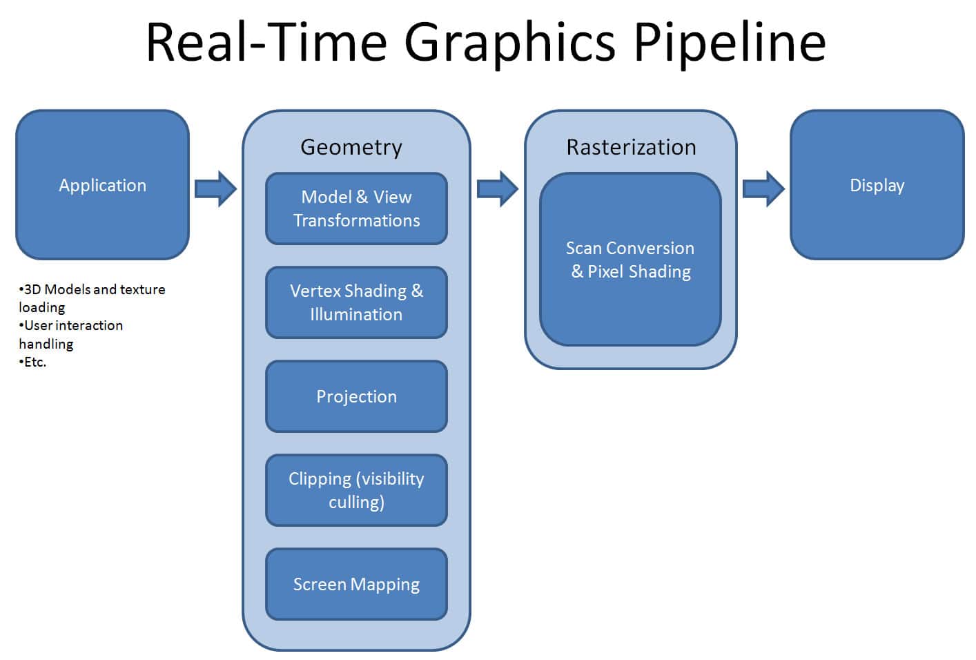
The graphics pipeline is a black box that transforms a geometric model of a scene and produces a pixel based perspective drawing of the real world onto the screen. The graphics pipeline is the path that data takes from the CPU, through the GPU, and out to the screen. Figure 1 describes a minimalist workflow of a graphics pipeline.
Every pixel passes through at least the following phases: vertices generation, vertex shading, generating primitives, rasterisation, pixel shading, testing and mixing. After all these stages, the pixel is sent to a frame buffer, which later results in the display of the pixel on the screen. This sequence is not a strict rule of how OpenGL is implemented but provides a reliable guide for predicting what OpenGL will do.
A list of vertices is fed into the GPU that will be put together to form a mesh. Information present with the vertices need not be restricted to its position in 3D space. If required, surface normals, texture coordinates, colours, and spatial coordinate values generated from the control points might also be associated with the vertices and stored. All data, whether it describes geometry or pixels, can be saved in a display list for current or later use.
The vertices that are processed are now connected to form the mesh. The GPU chooses which vertices to connect per triangle, based on either the order of the incoming vertices or a set of indices that maps them together. From vertex data, the next stage is the generation of primitives, which converts the vertices into primitives. Vertex data gets transformed by matrix transformations. Spatial coordinates are projected from the 3D space map onto a screen. Lighting calculations as well as generation and transformation of texture coordinates can take place at this stage.
Next comes clipping, or the elimination of portions of geometry which dont need to be rendered on the screen and are an overhead. Once we have figured out which pixels need to be drawn to the screen, the varying values from the vertex shader will be interpolated across the surface and fed into the pixel shader. These pixels are first unpacked from one of a variety of formats into the proper number of components. The colour of each pixel is determined. Now, we can use this information to calculate lighting, read from textures, calculate transparency, and use some high level algorithms to determine the depth of the pixels in 3D space.
We now have all the information that we need to map the pixels onto the screen. We can determine the colour, depth and transparency information of every single pixel, if needed. Its now the GPUs job to decide whether or not to draw the new pixels on the top of pixels already on the screen. Note that, prior to this stage, various complexities in the pipeline can occur. If textures are encountered, they have to be handled; if fog calculations are necessary, they are to be addressed. We can also have a few stencil tests, depth-buffer tests, etc. Finally, the thoroughly processed pixel information, the fragment’, is drawn into the appropriate buffer, where it finally advances to become a pixel and reaches its final resting place, the display screen.
Note that the above described fixed-pipeline model is now obsolete on modern GPUs, which have grown faster and smarter. Instead, the stages of the pipeline, and in some cases the entire pipeline, are being replaced by programs called shaders. This was introduced from OpenGL version 2.1 onwards. Modern 3D graphics programs have vertex shaders, evaluation shaders (tessellation shaders), geometry shaders, fragment shaders and compute shaders. Its easy to write a small shader that mimics what the fixed-function pipeline does, but modern shaders have grown increasingly complex, and they do many things that were earlier impossible to do on the graphics card. Nonetheless, the fixed-function pipeline makes a good conceptual framework on which to add variations, which is how many shaders are created.
Diving into OpenGL
As described, OpenGL is designed to be hardware-independent. In order to become streamlined on many different platforms, OpenGL specifications dont include creating a window, or defining a context and many other functions. Hence, we use external libraries to abstract this process. This helps us to make cross-platform applications and save the real essence of OpenGL.
The OpenGL states and buffers are collected by an abstract object, commonly called context. Initialising OpenGL is done by adding this context, the state machine that stores all the data that is required to render your application. When you close your application, the context is destroyed and everything is cleaned up.
The coding pattern these libraries follow is similar. We begin by specifying the properties of the window. The application will then initiate the event loop. Event handling includes mouse clicks, updating rendering states and drawing.
Heres how it looks:
#include <RequiredHeaders>

int main(){
createWindow();
createContext();

while(windowIsOpen){
while (event == newEvent()){
handleThatEvent(event);
}

updateScene();

drawRequiedGraphics();
presentGraphics();
}
return 0;
}
Coming to which libraries to use with OpenGL, we have a lot of options: https://www.opengl.org/wiki/Related_toolkits_and_APIs.
Here are a few noteworthy ones:
- The OpenGL Utility Library (GLU) provides many of the modelling features, such as quadric surfaces and NURBS curves and surfaces. GLU is a standard part of every OpenGL implementation.
- For machines that use the X Window System, the OpenGL Extension to the X Window System (GLX) is provided as an adjunct to OpenGL. The X Window System creates a hardware abstracted layer and provides support for networked computers.
- The OpenGL Utility Toolkit (GLUT) is a Window System-independent toolkit, which is used to hide the complexities of differing window system APIs. We will be using GLUT in our sample program.
- Mesa helps in running OpenGL programs on an X Window System, especially Linux.
- OpenInventor is a C++ 3D graphics API that abstracts on OpenGL.
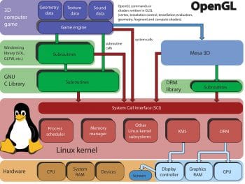
Now, let’s see what the workflow of a C++ OpenGL program looks like. We have our application program, the compiled code at one end. At the other end is a 3D image that is rendered to the screen.
Our program might be written with OpenInventor commands (or in native C++). The function calls are declared in OpenGL. These OpenGL calls are platform-independent. On an X Window System (like Linux), the OpenGL calls are redirected to the implementation calls defined by Mesa. The operating system might also have its own rendering API at this stage, which accelerates the rendering process. The OpenGL calls might also redirect to the implementation calls defined by the proprietary drivers (like Nvidia drivers, Intel drivers, etc, that facilitate graphics on the screen). Now, these drivers convert the OpenGL function calls into GPU commands. With its parallelism and speed, GPU maps the OpenGL commands into 3D images that are projected onto the screen. And this way we finally see 3D images called by OpenGL.
Setting up Linux for graphics programming
For graphics programming on a Linux machine, make sure that OpenGL is supported by your graphics cardalmost all of them do. OpenGL, GLX and the X server integration of GLX, are Linux system components and should already be part of the Debian, Red Hat, SUSE or any other distribution you use. Also make sure your graphics drivers are up to date. To update the graphics drivers on Ubuntu, go to System settings >> Software and Updates >> Additional drivers and install the required drivers.
Next, install GLUT. Download the GLUT source from http://www.opengl.org/resources/libraries/glut/glut_downloads.php and follow the instructions in the package. If youre programming in C++, the following files need to be included:
#include <GL/glut.h> // header file for the GLUT library
#include <GL/gl.h> // header file for the OpenGL32 library
#include <GL/glu.h> // header file for the GLu32 library
To execute this file, an OpenGL program, you require various development libraries like GL, GLU X11, Xrandr, etc, depending on the function calls used. The following libraries would be sufficient for a simple 3D graphics program. Use apt-get or yum to install these libraries:
freeglut3
freeglut3-dev
libglew1.5
libglew1.5-dev
libglu1-mesa
libglu1-mesa-dev
libgl1-mesa-glx
libgl1-mesa-dev
Next comes the linking part. You can use a Makefile to do this. But for our example, we will link them manually while compiling. Lets say we want to execute a C++ OpenGL program called main.cpp. We can link OpenGL libraries as follows:
g++ -std=c++11 -Wall -o main main.cpp -lglfw3 -lGLU -lGL -lX11 -lXxf86vm -lXrandr -lpthread -lXi
Note that the linking is done sequentially. So the order is important. You can now execute the program the usual way (./main for the above).
A simple OpenGL based example
Lets now write a minimal OpenGL program in C++. We will use GLUT for windowing and initialising context.
We have already discussed what an OpenGL based workflow looks like. We create a window, initialise a context, wait for some event to occur and handle it. For this simple example, we can ignore event handling. We will create a window and display a triangle inside it.
The required headers are:
#include <GL/glut.h> // header file for the GLUT library
#include <GL/gl.h> // header file for the OpenGL32 library
The latest versions of GLUT include gl.h. So we can only include the GLUT library header.
The main function will look like what follows:
int main (int argc, char** argv){
glutInit(&argc, argv);
// Initializing glut
glutInitDisplayMode(GLUT_SINGLE | GLUT_RGB);
// Setting up display mode, the single buffering and RGB colors glutInitWindowPosition(80, 80);
// Position of the window on the screen
glutInitWindowSize(400, 300);
// Size of the window
glutCreateWindow(A simple Triangle);
// Name of the window
glutDisplayFunc(display);
// The display function
glutMainLoop();
}
All the above are GLUT calls. Since OpenGL doesnt handle windowing calls, all the window creation is taken care of by GLUT. We initialise a window and set up the display mode. The display mode specified above states that the window should display RGB colours and will require a single buffer to handle pixel outputs. We then specify the window position on the screen, the size of the window to be displayed and the display function. The display function takes a pointer to a function as an argument. The function would describe what is to be displayed inside the screen. The final function call loops the main forever, so that the window is always open until closed.
Now that a window is initialised, lets draw a triangle with OpenGL function calls. Heres how the display function looks:
void display(){
glClear(GL_COLOR_BUFFER_BIT);
glBegin(GL_POLYGON);

glColor3f(1, 0, 0);
glVertex3f(-0.6, -0.75, 0.5);

glColor3f(0, 1, 0);
glVertex3f(0.6, -0.75, 0);

glColor3f(0, 0, 1);
glVertex3f(0, 0.75, 0);
glEnd();
glFlush();
}
All OpenGL based function calls begin with the letters gl in lowercase. We are planning to display a simple triangle defined by three vertices. We specify the colour and position of the vertices and map them on to the screen. For this, we first call the glClear() function which clears the display buffer. Next, we specify the type of primitive we are planning to draw with the glBegin() function. This is the primitive of our drawing until a glEnd() function is called. Next, between the glBegin() and glEnd() we draw three points (vertices) and form a triangle with them. We first have to specify the colour and then the position of the drawing. As OpenGL is platform independent, the C-style datatypes are specified as a function call. This can be seen with the glColor3f() function, which takes three float values.
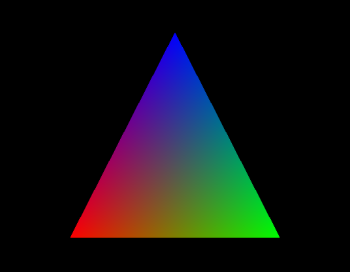
Once the program is compiled, linked and called as described above, it would look like whats shown in Figure 3.
If youre interested in learning OpenGL based computer graphics, the old version of the official red book is available for free at http://www.glprogramming.com/red/.


:)