This is the second article in the series on data analysis. The previous article dealt with pivot tables. This article explores ways to find the measures of central tendency and the measures of variability using MySQL.
Structured Query Language (SQL) is a good starting point for high level data analysis. Many data analysis packages and languages have their own interface to read data from different SQL based database systems. In fact, any real-life data analysis starts from an RDBMS, and the basic analysis and report generation is done on the SQL platform of that RDBMS itself. A good preview of data within the RDBMS platform itself helps analysts to get a fast high level analysis in a different platform. Besides this, since SQL can combine multiple tables, the export of compact data from different tables in a rich data analysis platform like R, Python or SPSS can make for a powerful data analysis system.
Here, I will discuss only the basic descriptive statistical data analysis facilities of SQL. Some of the options are implicitly available and some can be derived from the primary facilities of the language.
Resources
The analysis has been done on the Northwind RDBMS available in the Google archive (https://code.google.com/archive/p/northwindextended/downloads). Readers may download the data and can experiment with it in their own way.
Descriptive statistics
Data analysis is slightly different from general SQL based queries. While the basic purpose of the SQL query is to prepare a report, the purpose of data analysis is to analyse the report and come to a conclusion. As data analysis requires proper organisation of data in a particular context, an SQL query is an essential prerequisite. Data analysis is a vast and complex subject, and uses different supervised and unsupervised techniques. In this article, I will only cover the descriptive statistics to analyse data, in order to get some basic trends inherent to the distribution, so that an analyst can derive meaningful conclusions from the data and initiate a high level analysis of the data distributed over a set of tables.
For numerical data, descriptive statistics, in general, measures the central tendency (mean, median, mode) and the level of variability of the data. These measurements are a good starting point for data exploration and often lead to new questions that fuel further higher level analysis.
Most of the required analysis of data is the aggregation of data, as a whole or in groups. This is needed in order to have an overall view of the records. Aggregate functions allow us to easily produce summarised data from our database. With aggregation functions like MAX(), MIN(), AVG(),SUM() and COUNT() one can easily produce reports from database tables. Aggregate functions are all about performing the following:
- Calculations on multiple rows
- Calculations on a single column of a table
- Calculation to get a single value of a parameter
For instance, from the Northwind database, the management may require the following analysis reports:
- Least freight charge
- Most ordered items
- Average sales per month/per year
Measures of central tendency
Mean: The mean is the number you obtain when you sum up a given set of numbers and then divide this sum by the total number of samples in the set. The mean is very sensitive to outliers. It can be drastically affected by values that are much higher or lower compared to the rest of the data set.
Select b.ContactName,AVG(Freight)Freight from ordersasa
Join customers as b on a.CustomerID=b.CustomerID
Group by a.CustomerID;
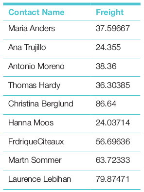 Median: The median is the number separating the higher half of an ordered data set from the lower half. Sometimes the median is a better choice of a mid-point because each data point is weighted equally with respect to the median value. Since MySQL doesn’t offer a built-in function to calculate the median value of a column, it is necessary to build a query of our own.
Let us assume that we want to retrieve the median value of the column quantity from the table orderitem as shown below:
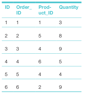 Let’s look into the algorithm we’re going to use to build the query.
- Retrieve a sorted list of the values from column Quantity and attach an index to each row.
- In case of an odd number of values in the column, find the value of the item in the middle of the sorted list.
- In case of an even number of values in the column, find the values of the two items in the middle of the sorted list.
- Calculate the average of the value(s) retrieved in these steps.
- Return the average value as the median value.
1. SET @rowindex:=-1;
2. SELECT
3. Order_ID,rowindex,AVG(Quantity)as Median
4. FROM
5. (SELECTOrder_ID,@rowindex:=@rowindex+1 AS rowindex,
6. orderitem.Quantity AS Quantity
7. FROM orderitem
8. ORDER BYorderitem.Quantity) AS g
9. WHERE
10. g.rowindexIN(FLOOR(@rowindex/2),CEIL(@rowindex/2))
 Since there are even numbers of items, the median is an average of two middle values. The query structure is a little complex. To get a better understanding of the above query, we can explore the sub-query (lines 5-8) of the FROM clause of the above query.
1. SET@rowindex:=-1;
2. SELECTOrder_ID,@rowindex:=@rowindex+1ASrowindex,
3. orderitem.QuantityASQuantity
4. FROMorderitem
5. ORDERBYorderitem.Quantity
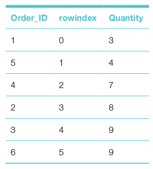 The output table of the sub-query shows that the median value will be between 7 and 8.
Mode: The mode is the value that appears most often in a set of data. To find the mode of the quantity of the table orderitem we can write the mode query as follows:
Mode query

SELECT
orderitem.quantity,
COUNT(*) as count
FROM orderitem
Group by orderitem.quantity
ORDER BY COUNT(*) DESC
LIMIT1
The GROUP BY clause provides a count of the items in each group and the ORDER BY clause provides, in descending order, the maximum (mode) count value at the top. The LIMIT clause isolates the mode at the top of the column Quantity.
If the contents of the orderitem table are as follows:
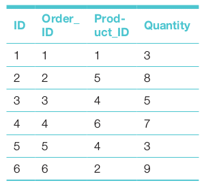 Then the mode-query will return the following:
 Measures of variability
In statistics, variability is the extent to which a distribution is extended or squeezed. Common examples of measures of statistical variability are the max., min., variance, standard deviation, and interquartile ranges.
Max. and min: The maximum and minimum values of any numerical field of a table can be reported in a tabular form by the aggregation functions max and min of MySQL. To find the max and min freight values of the invoice table of the Northwind database, the SQL query can be written as follows:
Variability
SELECT
MAX(freight) as MAX_freight,MIN(freight) as MIN_freight
FROMinvoices;
Standard deviation: Standard deviation is a measure of the spread of values in a data set. It shows the extent of variation of data from the average (mean). A low standard deviation shows that the values in the data set are close to the mean, while a high standard deviation indicates that the values of the data set are spread out over a large range of values.
MySQL supports both the population and sample standard deviations. There are a few variations among different functions, regarding which readers may consult documents.
STD(field) returns the population standard deviation of the expression and returns NULL if there is no matching row:
use northwind;
select format(std(freight),2) as Pop_STD
from orders as t
where customerID=’VINET’
order by customerID;

Output of population standard deviation:
10.84
STDDEV_SAMP(field) returns the sample standard deviation:
use northwind;
select format(STDDEV_SAMP(freight),2) as Pop_STD
from orders as t
where customerID=’VINET’
order by customerID;


Output sample standard deviation:
12.11
The population and sample standard deviations of freight charges of the customer Vinet are shown in the above two code snippets.
MySQL also has functions for population variance and sample variance calculations. These are:
- VAR_POP(field), which calculates the population standard variance of the field.
- VARIANCE(field), which is the same as VAR_POP function.
- VAR_SAMP(field), which calculates the sample standard variance of the field.
Distribution pattern
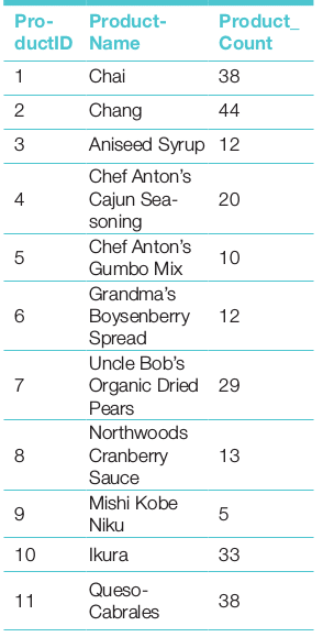
Distribution of data plays an important role in statistical data analysis. The histogram is an important statistical tool to understand the distribution pattern. The count of items in each group can be done by count() of the target item using the GROUP_BY clause. This is shown in the following query:
SELECT
a.productID,b.ProductName,count(a.productID) as Product_Count
FROM invoices as a
Join products as b on a.ProductID=b.ProductID
Group by a.productID
Order bya.productID;
The Frequency table is given below.