


We have covered a lot of material in the R programming language syntax such as data structures, and import and transformation of data. In this sixth article in the ‘R, Statistics and Machine Learning’ series, we shall explore the various user interfaces available to interact with R.
We will be using R version 4.1.0 installed on Parabola GNU/Linux-libre (x86-64) for the code snippets.
$ R --version
R version 4.1.0 (2021-05-18) -- “Camp Pontanezen”
Copyright (C) 2021 The R Foundation for Statistical Computing
Platform: x86_64-pc-linux-gnu (64-bit)
R is free software and comes with absolutely no warranty. You are welcome to redistribute it under the terms of the GNU General Public License versions 2 or 3. For more information on these matters, see https://www.gnu.org/licenses/.
R console
We have already used the R console environment to learn the semantics of the R programming language. The console provides a REPL (Read-Eval-Print Loop) to iteratively develop software, and is very useful when experimenting or testing code. You can start an R console session using the R command, and it will provide a prompt. You can exit the session using the quit() function as shown below:
$ R
R version 4.1.0 (2021-05-18) -- “Camp Pontanezen”
Copyright (C) 2021 The R Foundation for Statistical Computing
Platform: x86_64-pc-linux-gnu (64-bit)
R is free software and comes with ABSOLUTELY NO WARRANTY.
You are welcome to redistribute it under certain conditions.
Type ‘license()’ or ‘licence()’ for distribution details.
   Natural language support but running in an English locale
R is a collaborative project with many contributors.
Type ‘contributors()’ for more information and
‘citation()’ on how to cite R or R packages in publications.
 Type ‘demo()’ for some demos, ‘help()’ for on-line help, or
‘help.start()’ for an HTML browser interface to help.
Type ‘q()’ to quit R.
> quit()
Save workspace image? [y/n/c]: n
The command line R execution supports multiple arguments, as can be seen from the help option:
$ R --help$ R --help
The output of the command will be displayed on your screen with all the details.
Batch mode
R provides a batch mode, where you can script a series of commands from a source file. For example, we can write a script to read the bank.csv file from the ‘Bank Marketing Data Set’ available from the UCI machine learning repository available at https://archive.ics.uci.edu/ml/datasets/Bank+Marketing. You can display the first few rows and print a summary of the data in the following batch.R file:
bank <- read.csv(file=”bank.csv”, sep=”;”)
head(bank)
print(summary(bank))
You can execute the script using the following command from a bash shell prompt:
$ R CMD BATCH batch.R
By default, the results are stored in a .Rout file. The time taken to run the script is also recorded in the output.
$ cat batch.Rout
R version 4.1.0 (2021-05-18) -- “Camp Pontanezen”
Copyright (C) 2021 The R Foundation for Statistical Computing
Platform: x86_64-pc-linux-gnu (64-bit)
R is free software and comes with ABSOLUTELY NO WARRANTY.
You are welcome to redistribute it under certain conditions.
Type ‘license()’ or ‘licence()’ for distribution details.
  Natural language support but running in an English locale
R is a collaborative project with many contributors.
Type ‘contributors()’ for more information and
‘citation()’ on how to cite R or R packages in publications.
Type ‘demo()’ for some demos, ‘help()’ for on-line help, or
‘help.start()’ for an HTML browser interface to help.

Type ‘q()’ to quit R.
[Previously saved workspace restored]
> bank <- read.csv(file=”bank.csv”, sep=”;”)
>
> head(bank)
  age         job marital education default balance housing loan  contact day
1 30  unemployed married  primary  no 1787 no  no cellular 19
2  33 services married secondary no 4789 yes yes cellular  11
3  35  management single tertiary no 1350 yes no cellular  16
4  30  management married tertiary no 1476 yes yes unknown  3
5  59 blue-collar married secondary no 0  yes no  unknown   5
6  35  management  single  tertiary no 747 no no cellular  23
  month duration campaign pdays previous poutcome  y
1   oct       79        1    -1        0  unknown no
2   may      220        1   339        4  failure no
3   apr      185        1   330        1  failure no
4   jun      199        4    -1        0  unknown no
5   may      226        1    -1        0  unknown no
6   feb      141        2   176        3  failure no
>
> print(summary(bank))
      age            job              marital           education
 Min.  :19.00  Length:4521     Length:4521       Length:4521
 1st Qu.:33.00 Class :character Class :character Class :character
 Median :39.00   Mode  :character   Mode  :character   Mode  :character
 Mean   :41.17
 3rd Qu.:49.00
 Max.   :87.00
   default             balance        housing              loan
 Length:4521        Min.   :-3313   Length:4521        Length:4521
 Class :character   1st Qu.:   69   Class :character   Class :character
 Mode  :character   Median :  444   Mode  :character   Mode  :character
                    Mean   : 1423
                    3rd Qu.: 1480
                    Max.   :71188
   contact         day           month              duration
 Length:4521     Min.  : 1.00   Length:4521        Min.   :   4
 Class :character  1st Qu.: 9.00  Class :character 1st Qu.: 104
 Mode  :character Median :16.00   Mode :character  Median : 185
                Mean   :15.92                 Mean   : 264
                3rd Qu.:21.00                 3rd Qu.: 329
				Max.   :31.00                      Max.   :3025
    campaign        pdays       previous        poutcome
 Min.   : 1.000   Min.   : -1.00   Min.   : 0.0000   Length:4521
 1st Qu.: 1.000   1st Qu.: -1.00   1st Qu.: 0.0000   Class :character
 Median : 2.000   Median : -1.00   Median : 0.0000   Mode  :character
 Mean   : 2.794   Mean   : 39.77   Mean   : 0.5426
 3rd Qu.: 3.000   3rd Qu.: -1.00   3rd Qu.: 0.0000
 Max.   :50.000   Max.   :871.00   Max.   :25.0000
      y
 Length:4521
 Class :character
 Mode  :character

>
> proc.time()
   user  system elapsed
  0.160   0.036   0.144
You can also use the Rscript command to execute the above script, as shown below:
$ Rscript batch.R
The R commands can also be written to a source file with the shebang (“#!”) operator. For example:
#! /usr/bin/env Rscript
print(“From executable Rscript!”);
The script can be executed as follows:
$  ./batch_print.R
[1] “From executabl
GNU Emacs
The Emacs Speaks Statistics (ESS) package provides support to work with statistical packages. It also has support to work with R code and GNU Emacs. You can add the following to your Cask file, and install the ESS package:
(depends-on “ess”)
You can add the following to your GNU Emacs initialisation file in order to use the R mode support:
(require ‘ess-r-mode)
The M-x ess-version command provides the installed version number, which is 20211204.958 from the ELPA repository on GNU Emacs 27.2. You can start an R session from Emacs using M-x R. Emacs will prompt for a starting working directory, and a new buffer with an R prompt will be displayed, as shown below:
R version 4.1.0 (2021-05-18) -- “Camp Pontanezen”
Copyright (C) 2021 The R Foundation for Statistical Computing
Platform: x86_64-pc-linux-gnu (64-bit)
R is free software and comes with ABSOLUTELY NO WARRANTY.
You are welcome to redistribute it under certain conditions.
Type ‘license()’ or ‘licence()’ for distribution details.
  Natural language support but running in an English locale
R is a collaborative project with many contributors.
Type ‘contributors()’ for more information and
‘citation()’ on how to cite R or R packages in publications.
Type ‘demo()’ for some demos, ‘help()’ for on-line help, or
‘help.start()’ for an HTML browser interface to help.
Type ‘q()’ to quit R.
> setwd(‘/home/guest/working/’)
>
A number of commands have been implemented to interact between R code and the ESS process. A summary of the available commands to evaluate code is given in Table 1.
| Command | Comments |
| ess-eval-region-or-line-and-step | Evaluate highlighted region or current line and step to next line of code |
| ess-eval-region-or-function-or-paragragh | Send selected region or function or paragraph |
| ess-eval-line | Send current line |
| ess-eval-line-and-go | Send line and switch point to the ESS process |
| ess-eval-function | Send function |
| ess-eval-function-and-go | Send function and switch point to the ESS process |
| ess-eval-buffer | Send the current buffer |
| ess-eval-buffer-and-go | Send current buffer and switch point to the ESS process |
The advantage of using an R session within GNU Emacs is that you can save the session for future reference. You can also use ESS with the TRAMP (transparent remote access, multiple protocols) package to start a remote session. The same can be initiated with the ess-remote command. Do read the ‘ESS – Emacs Speaks Statistics’ PDF manual to learn more about its use.
The Babel project provides the ability to execute R code in an Emacs org file. The following code snippet enables support for R Babel and needs to be included in the Emacs initialisation file:
(org-babel-do-load-languages
‘org-babel-load-languages
‘((R . t)))
You can enclose R code within the org Babel code blocks and execute the same in an Emacs org file to obtain the results as shown below:
#+BEGIN_SRC R
1 < 2
#+END_SRC

#+RESULTS:
: TRUE
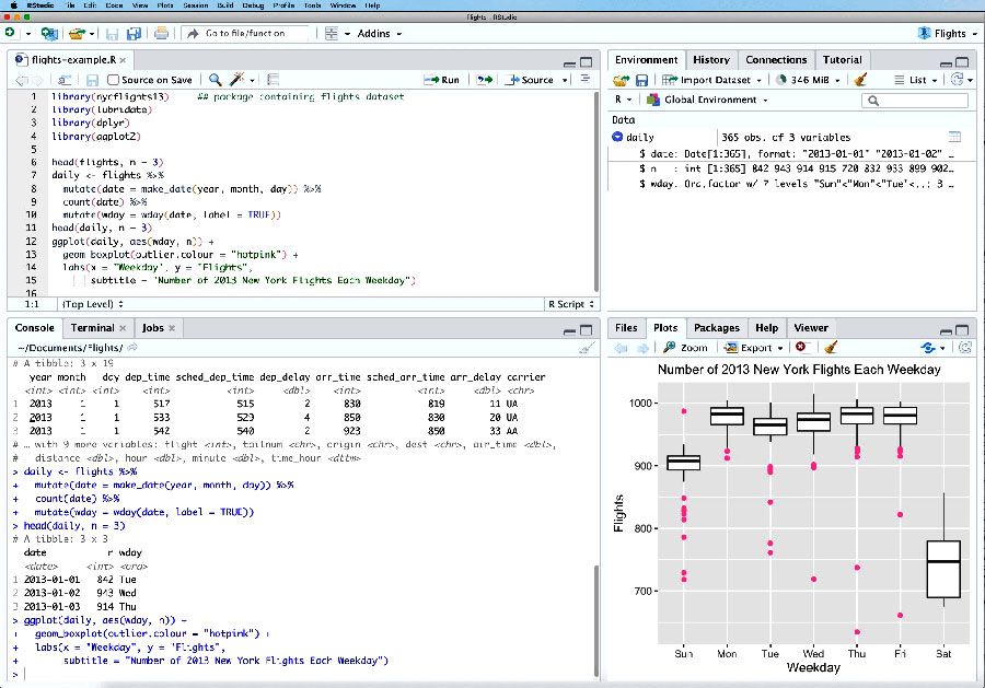
RStudio
RStudio is an integrated development environment (IDE) for the R programming language. It can be used as a desktop application, as well as a server that can be accessed on a browser. It is primarily written in Java, C++ and JavaScript, and the open source edition is available at https://github.com/rstudio/rstudio. Refer to Figure 1 for RStudio.
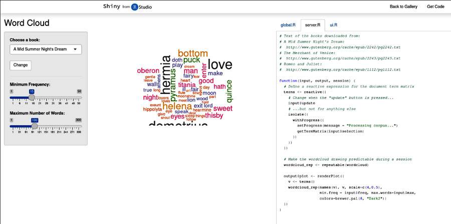
Shiny
Shiny is an R package that is useful to develop interactive Web applications with R. You can install it with your R environment using:
> install.packages(“shiny”)
...
* installing *source* package ‘shiny’ ...
** package ‘shiny’ successfully unpacked and MD5 sums checked
** using staged installation
 ** R
** inst
** byte-compile and prepare package for lazy loading
** help
*** installing help indices
*** copying figures
** building package indices
** testing if installed package can be loaded from temporary location
** testing if installed package can be loaded from final location
** testing if installed package keeps a record of temporary installation path
* DONE (shiny)
There are pre-built examples and demos provided by the installed Shiny package. You can test one of the examples using the following commands:
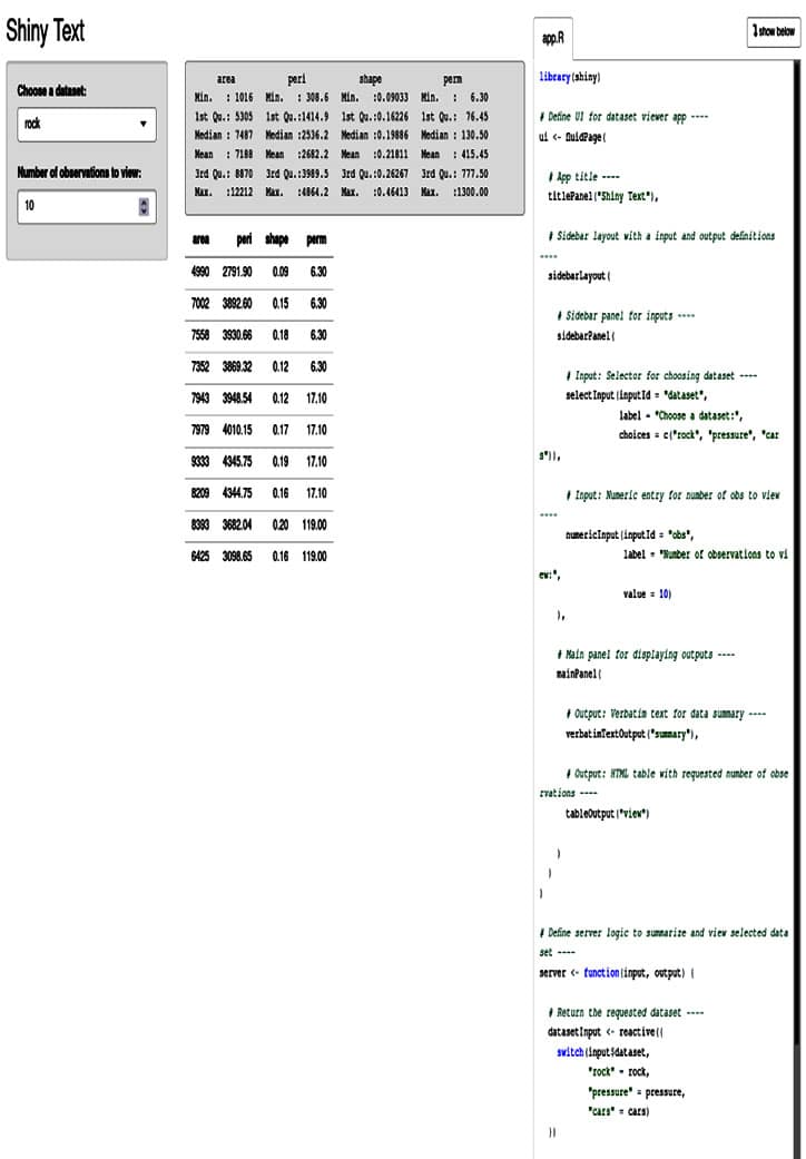
> library(shiny)
> runExample(“02_text”)
 Listening on http://127.0.0.1:3535
The app listens on a port and you need to set the default R browser in /etc/R/Renviron. For example, on Parabola GNU/Linux-libre, the setting is updated to use the Iceweasel (Firefox) browser as follows:
## Default browser
R_BROWSER=${R_BROWSER-’/usr/bin/iceweasel’}
The source code for the app defines the user interface and the server logic. A fluid layout is used for the panel, and the input selection consists of drop-down menus and text boxes. The server logic uses a reactive programming style to handle the input and displays the data.
library(shiny)
# Define UI for dataset viewer app ----
ui <- fluidPage(
  # App title ----
  titlePanel(“Shiny Text”),
  # Sidebar layout with a input and output definitions ----
  sidebarLayout(
    # Sidebar panel for inputs ----
    sidebarPanel(
      # Input: Selector for choosing dataset ----
      selectInput(inputId = “dataset”,
                  label = “Choose a dataset:”,
                  choices = c(“rock”, “pressure”, “cars”)),
      # Input: Numeric entry for number of obs to view ----
      numericInput(inputId = “obs”,
                   label = “Number of observations to view:”,
                   value = 10)
    ),
    # Main panel for displaying outputs ----
    mainPanel(
      # Output: Verbatim text for data summary ----
      verbatimTextOutput(“summary”),
      # Output: HTML table with requested number of observations ----
      tableOutput(“view”)
    )
  )
)
# Define server logic to summarize and view selected dataset ----
server <- function(input, output) {
  # Return the requested dataset ----
  datasetInput <- reactive({
    switch(input$dataset,
           “rock” = rock,
           “pressure” = pressure,
           “cars” = cars)
  })
  # Generate a summary of the dataset ----
  output$summary <- renderPrint({
    dataset <- datasetInput()
    summary(dataset)
  })
  # Show the first “n” observations ----
  output$view <- renderTable({
    head(datasetInput(), n = input$obs)
  })
}
# Create Shiny app ----
shinyApp(ui = ui, server = server)
It is recommended to go through the Shiny tutorial videos and the code examples to learn how to best use Shiny for your data sets.


