


Discover how the Bag-of-Words model can be applied and visualised in a Python project.
The Bag-of-Words (BoW) model is a fundamental technique for text processing and natural language processing (NLP). It considers each word as an integer number and assigns the frequency of its occurrences within a document constituting the corpus. In Python, the Gensim library provides powerful tools to work with BoW models, including the ‘corpora.Dictionary’ class. In rule-based NLP, BoW is an intermediate stage where it receives data from the preliminary text processing steps like cleaning, removal of stopwords and punctuations, and so on, and then provides this data for high-level analysis to understand the corpus. Let’s explore how the BoW approach is applied and visualised in a Python project.
The corpora.Dictionary class in Gensim is a mapping between words and their integer IDs. It helps to create the BoW representation of text documents, which is essential for many NLP tasks, including topic modelling.
You can create a dictionary as follows:
import numpy as np
from gensim import corpora
#Sample preprocessed texts
texts = [[“PHI”, “EWP”,”PHI”],[“EWP”,”Elsevier”],[“PHI”,”Elsevier”,”EWP”]]
dictionary = corpora.Dictionary(texts)
#Display the dictionary **
print(dictionary.token2id)

## {‘EWP’: 0, ‘PHI’: 1, ‘Elsevier’: 2}
Creating the Bag-of-Words (BoW) model
The BoW model represents each document as a list of word IDs and their corresponding frequencies. This can be achieved using the doc2bow() method. Here’s an example:
bow_corpus = [dictionary.doc2bow(text) for text in texts]
print(bow_corpus)

## [[(0, 1), (1, 2)], [(0, 1), (2, 1)], [(0, 1), (1, 1), (2, 1)]]
This bag of words can be easily understood by using a for-next-loop to see each word’s document-wise frequency:
# Print corpus
for i, doc in enumerate(bow_corpus):
print(f”Document {i+1}: {doc}”)

## Document 1: [(0, 1), (1, 2)]
## Document 2: [(0, 1), (2, 1)]
## Document 3: [(0, 1), (1, 1), (2, 1)]
To process a corpus, the most important step is to have a list of words of the corpus vocabulary, as corpora.Dictionary() creates a dictionary, i.e., unique (key, value) pairs from the corpus.
#Corpus Dictionary
vocabulary = [dictionary[id] for id in dictionary.keys()]
print(vocabulary)

## [‘EWP’, ‘PHI’, ‘Elsevier’]
This vocabulary-frequency extraction from a corpus is a great achievement for further high-level processing of a corpus. A word-frequency table can be programmed from the bow_corpus and dictionary, and convert the counter outcome to a DataFrame.
from collections import Counter
word_counts = Counter()
for doc in bow_corpus:
for word_id, freq in doc:
word = dictionary[word_id]
word_counts[word] += freq
print(word_id,freq,word,word_counts[word])

## 0 1 EWP 1
## 1 2 PHI 2
## 0 1 EWP 2
## 2 1 Elsevier 1
## 0 1 EWP 3
## 1 1 PHI 3
## 2 1 Elsevier 2

print(‘Type of word_counts: ‘,word_counts)

## Type of word_counts: Counter({‘EWP’: 3, ‘PHI’: 3, ‘Elsevier’: 2})
Using a Pandas DataFrame, a counter data type can easily be converted to a DataFrame for easy and elegant visualisation. This will give us a word-frequency table.
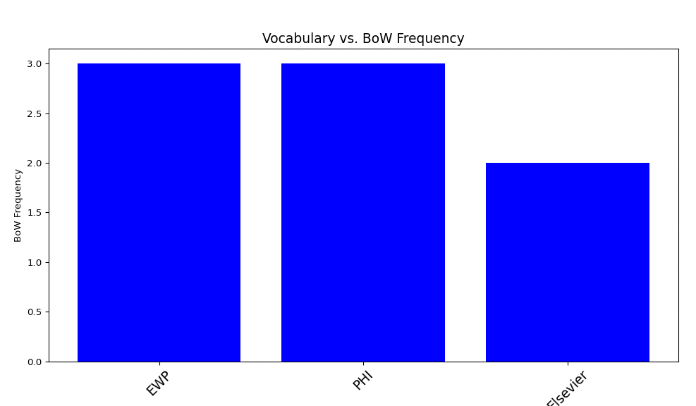
# Convert to a DataFrame for easier visualization
import pandas as pd
df = pd.DataFrame(word_counts.items(), columns=[‘Word’, ‘Frequency’])
df = df.sort_values(by=’Frequency’, ascending=False)
#Word frequency table
print(df)

## Word Frequency
## 0 EWP 3
## 1 PHI 3
## 2 Elsevier 2
Finally, matplotlib may be used to create a word-frequency plot of the corpus vocabulary in the manner described below:
# Plotting the frequency graph
import matplotlib.pyplot as plt
plt.figure(figsize=(12, 6))
plt.bar(df[‘Word’], df[‘Frequency’], color= ‘blue’) # Show top 20 words
plt.title(‘Vocabulary vs. BoW Frequency’,fontsize = 14)
plt.xlabel(‘Vocabulary’)
plt.ylabel(‘BoW Frequency’)
plt.xticks(rotation=45,fontsize = 14)

## ([0, 1, 2], [Text(0, 0, ‘EWP’), Text(1, 0, ‘PHI’), Text(2, 0, ‘Elsevier’)])

plt.show()
Complete Python code for the vocabulary study of a corpus consisting of four texts has been discussed here. Before the processing for vocabulary extraction, the entire corpus has been tokenised to clean with respect to stopwords, punctuation, and some special words like ‘is’, ‘the’ and ‘of’. Then, to normalise the vocabulary of the corpus, a dictionary-based lemmatization has been used with the Python module spaCy.
from gensim import corpora, models
from nltk.corpus import stopwords
from nltk.tokenize import word_tokenize
from nltk.stem import PorterStemmer
import string
import nltk
import spacy
import matplotlib.pyplot as plt
import pandas as pd
from collections import Counter
nltk.download(‘punkt_tab’)
## False
nlp = spacy.load(“en_core_web_sm”)
documents = [ “Knowledge of statistics is essential for data analysis.”,
“The concept of statistics is also helpful for economics.”
“The idea of economics is essential for social study.” ,
“Data analysis is an essential part of machine learning.”
]
# Tokenization
texts = [word_tokenize(doc.lower()) for doc in documents]
# Remove punctuation
words_no_punct = [word for lstitm in texts for word in lstitm if word not in string.punctuation]
# Remove stopwords
process_corpus = []
alist = []
for list_word in texts:
for listitm in list_word:
if listitm not in string.punctuation:
alist.append(listitm)
process_corpus.append(alist)
alist=[]
# Remove “is” “the”, “of”
process_corpus2 = []
alist = []
for list_word in process_corpus:
for listitm in list_word:
if listitm not in [‘is’, ‘the’,’of’]:
alist.append(listitm)
process_corpus2.append(alist)
alist=[]
# Remove stopwords
stopwords = set (stopwords.words(“english”))
vocabulary = set()
v = []
alist = []
for list_word in process_corpus2:
for listitm in list_word:
if listitm not in stopwords:
alist.append(listitm)
v.append(alist)
vocabulary.update(alist)
alist=[]
# Convert to a sorted list
vocabulary = sorted(list(vocabulary))
print(“Vocabulary:”, vocabulary)
## Vocabulary: [‘also’, ‘analysis’, ‘concept’, ‘data’, ‘economics’, ‘economics.the’, ‘essential’, ‘helpful’, ‘idea’, ‘knowledge’, ‘learning’, ‘machine’, ‘part’, ‘social’, ‘statistics’, ‘study’]
filtered_doc = [token.lemma_ for token in nlp(“ “.join(vocabulary))]
# Create a dictionary and corpus
filtered_doc = [filtered_doc]
dictionary = corpora.Dictionary(filtered_doc)
print(“Token to id: “,dictionary.token2id)
## Token to id: {‘also’: 0, ‘analysis’: 1, ‘concept’: 2, ‘datum’: 3, ‘economic’: 4, ‘economics.the’: 5, ‘essential’: 6, ‘helpful’: 7, ‘idea’: 8, ‘knowledge’: 9, ‘learn’: 10, ‘machine’: 11, ‘part’: 12, ‘social’: 13, ‘statistic’: 14, ‘study’: 15}
corpus = [dictionary.doc2bow(text) for text in texts]
print(“Corpus: “,corpus,’\n’)
## Corpus: [[(1, 1), (6, 1), (9, 1)], [(0, 1), (2, 1), (5, 1), (6, 1), (7, 1), (8, 1), (13, 1), (15, 1)], [(1, 1), (6, 1), (11, 1), (12, 1)]]
# Print corpus
for i, doc in enumerate(corpus):
print(f”Document {i+1}: {doc}”)
print(‘\n’)
## Document 1: [(1, 1), (6, 1), (9, 1)]
##
##
## Document 2: [(0, 1), (2, 1), (5, 1), (6, 1), (7, 1), (8, 1), (13, 1), (15, 1)]
##
##
## Document 3: [(1, 1), (6, 1), (11, 1), (12, 1)]
# Prepare frequency table
vocabulary2 = [dictionary[id] for id in dictionary.keys()]
# Flatten the corpus to count word frequencies
word_counts = Counter()
for doc in corpus:
for word_id, freq in doc:
word = dictionary[word_id]
word_counts[word] += freq
print(word_id,freq,word,word_counts[word])
## 1 1 analysis 1
## 6 1 essential 1
## 9 1 knowledge 1
## 0 1 also 1
## 2 1 concept 1
## 5 1 economics.the 1
## 6 1 essential 2
## 7 1 helpful 1
## 8 1 idea 1
## 13 1 social 1
## 15 1 study 1
## 1 1 analysis 2
## 6 1 essential 3
## 11 1 machine 1
## 12 1 part 1
# Convert to a DataFrame for easier visualization
df = pd.DataFrame(word_counts.items(), columns=[‘Word’, ‘Frequency’])
df = df.sort_values(by=’Frequency’, ascending=False)
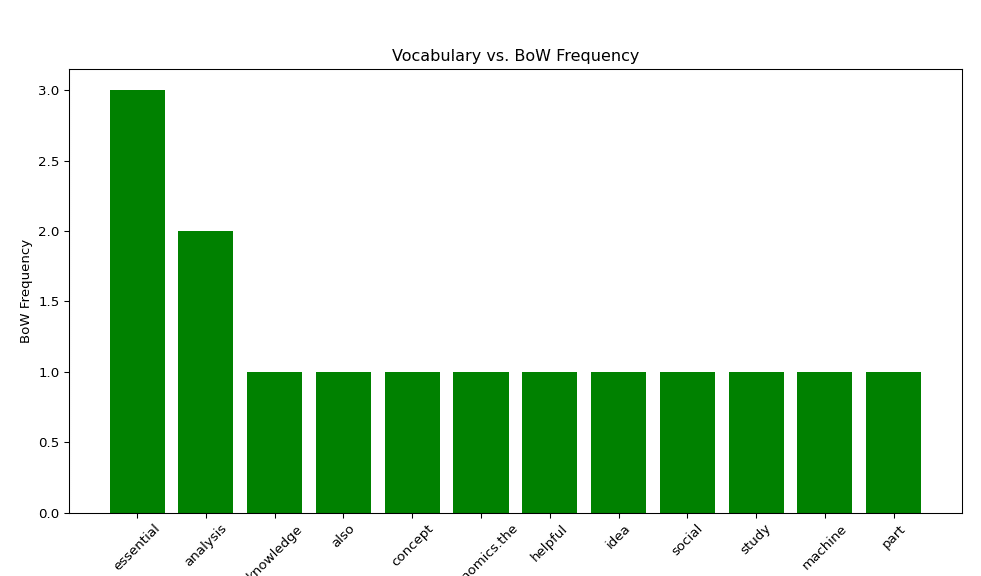
# Plotting the frequency graph
plt.figure(figsize=(12, 6))
plt.bar(df[‘Word’], df[‘Frequency’],color = ‘green’) # Show top 20 words
plt.title(‘Vocabulary vs. BoW Frequency’,fontsize=12)
plt.xlabel(‘Vocabulary’)
plt.ylabel(‘BoW Frequency’)
# set font size for both major and minor ticks
plt.xticks(rotation=45,fontsize = 10)
## ([0, 1, 2, 3, 4, 5, 6, 7, 8, 9, 10, 11], [Text(0, 0, ‘essential’), Text(1, 0, ‘analysis’), Text(2, 0, ‘knowledge’), Text(3, 0, ‘also’), Text(4, 0, ‘concept’), Text(5, 0, ‘economics.the’), Text(6, 0, ‘helpful’), Text(7, 0, ‘idea’), Text(8, 0, ‘social’), Text(9, 0, ‘study’), Text(10, 0, ‘machine’), Text(11, 0, ‘part’)])
plt.show()
As can be seen, the corpus’s vocabulary and word frequency are provided by the BoW model in conjunction with corpora.Dictionary. Additionally, it associates words with their integer identification numbers, which serves as the foundation for text processing and advanced corpus comprehension.


