


Discover how Python, a language most programmers love, is also turning into the language of choice for developing machine learning models.
As we all know, machine learning (ML) automates decision-making while Python is a simple language with a clean syntax and numerous libraries. What’s interesting is that Python has evolved with the times and is now the language of choice for machine learning. Before we find out why this is so, let’s get acquainted with the basic programming components of Python used for machine learning.
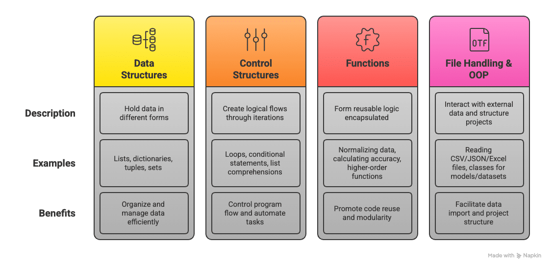
Central to everything in Python are data structures — the lists, dictionaries, tuples, sets, etc, used to hold data in different forms. Lists are for ordered collections of items that can be iterated over and for mapping keys to the values-dictionary, an important aspect of labelled datasets; tuples provide immutability, useful in contexts where data integrity is critical; and sets deal with unique features — for instance, removing duplicates from a dataset.
Control structures include loops and conditional statements, and they allow logical flows and iterations over data. For example, you may need to loop through a dataset to clean missing values or apply a custom transformation to each record. List comprehensions provide an elegant and direct Pythonic way to accomplish this, enhancing readability and reducing lines of code. Functions in Python allow forming the reusable logic encapsulated in them. For instance, whether we are talking about a function that normalises data or calculates accuracy, modular code with parameters and return values is what defines machine learning workflows. Also, higher-order functions in Python accept other functions as arguments, which is handy when filters or transformations are applied over datasets.
Working with files and external data is also fundamental in machine learning. Python’s file handling capabilities, coupled with reading from CSV, JSON, and Excel files, help import data from different sources. With its advanced bulk functions for reading and manipulating tabular data, Pandas also makes this task simpler. Even though it is not strictly required for simple ML tasks, a knowledge of OOP or object-oriented programming is helpful in larger projects. The fact that classes are defined for models, datasets, or preprocessing pipelines leads to cleaner and more maintainable code.
Python libraries used in ML
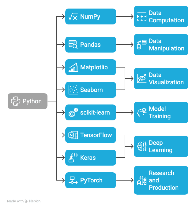
A prime reason why Python is an unrivalled choice for machine learning is the powerful set of libraries associated with it. These libraries abstract complex mathematical operations into simple APIs for building, training, and deploying models.
NumPy: NumPy or Numerical Python is considered the fundamental package for scientific computation in Python. It supports high-performance multidimensional arrays and matrices, along with a few functions to operate on them. In machine learning, NumPy serves as the backbone for most computations ranging from vectorized operations to linear algebra.
Pandas: Pandas is the main library for data manipulation and analysis, and it introduces two core data structures, namely, Series and Data Frame, which make it simple to load and explore as well as clean and transform data. Etiquette handles missing values, filters out rows, aggregates statistics, etc, quite rapidly and intuitively. Pandas is a must in the first stages of any machine learning pipeline.
Matplotlib and Seaborn: Visualisation is paramount in trying to understand the patterns and relationships that reside within data. Matplotlib is a low-level plotting library, while Seaborn builds on top of it, providing high-level representations of statistical plots. Such tools help the developer in making histograms, box plots, scatter plots, and correlation matrices to present data in an effective manner.
scikit-learn: scikit-learn is one of the most popular libraries in classical machine learning. It provides a consistent interface for model training, feature selection, data splitting, and evaluation of the model performance. From regression and classification, to clustering and dimensionality reduction, scikit-learn aims to ease implementation with clean, simple, and consistent APIs.
TensorFlow and Keras: TensorFlow is a widely used library developed by Google for numerical computation and deep learning. It can build highly sophisticated neural network architectures and supports training as well as inferences on CPU, GPU, or TPU. Slightly advanced in terms of the UI, Keras comes with TensorFlow and allows for better prototyping and experimentation.
PyTorch: PyTorch’s dynamic computation graphs and flexibility were developed by the AI Research Lab of Facebook, making it a highly acclaimed library, especially in academia and research. However, PyTorch can also be deployed in production systems, where it is supported by additional libraries like TorchServe.
Core Python concepts for machine learning
|
Concept |
Description |
Use in ML |
Basic code example |
|
Lists |
Ordered, mutable collections of items |
Store sequences of values like feature vectors or predictions. |
features = [0.2, 0.4, 0.9] |
|
Dictionaries |
Key-value pairs for fast data lookup |
Store dataset records, label mappings, or configuration parameters. |
labels = {‘cat’: 0, ‘dog’: 1} |
|
Tuples |
Ordered, immutable collections |
Represent fixed-size data like coordinates or hyperparameter sets. |
coords = (45.0, 90.0) |
|
Sets |
Unordered collections of unique elements |
Remove duplicates from data or compare feature sets. |
unique_words = set(word_list) |
|
Functions |
Reusable blocks of code defined with def |
Encapsulate repeated logic (e.g., data cleaning, metric calculation). |
def normalize(data): … |
|
Loops |
for and while loops to iterate through data |
Iterate over datasets, apply transformations, or train over epochs. |
for x in data: process(x) |
|
List comprehensions |
Compact syntax for generating lists from iterable objects |
Efficiently transform or filter data in a single line. |
[x**2 for x in range(5)] |
|
Files |
File handling with open(), read(), write() |
Read datasets from text, CSV, or JSON formats. |
with open(‘data.csv’) as f: … |
|
Modules |
Import reusable code from Python files or standard libraries |
Organise code, use external libraries like NumPy, scikit-learn, etc. |
import pandas as pd |
Key steps in a machine learning pipeline
Machine learning modelling is complicated and structured. Some of the critical steps in a typical machine learning pipeline are outlined below, illustrated with the relevant code examples.
Data collection
The first step in any machine learning pipeline is data collection. Machine learning models depend largely on data to acquire their patterns and make predictions. Without high-quality, representative data, predictions from the model could be wrong or irrelevant. Data is collected from various sources — structured databases, raw files like CSV or Excel, or any API to fetch real-time data.
After the data is collected, it is important to check for its quality and relevance to the task at hand. In other words, if you are working on a classification task to predict customer churn, the dataset must include relevant features like customer behaviour, demographics, and purchase history. Python tools generally used for loading and exploring the datasets are Pandas and NumPy, which have the best support for operating and manipulating structured data.
import pandas as pd
# Reading data from a CSV file
df = pd.read_csv(‘data.csv’)
# Displaying the first few rows of the data
print(df.head())
Data preprocessing
Raw data is often incomplete or inconsistent, and must be cleaned and prepared for training. Incomplete data can also lead to predictions that are biased. Hence, the first concern is missing data. Data with missing values can be deleted or an estimated value can be added. The second concern is the conversion of categorical variables into a numerical format because most machine learning algorithms require a numerical input. The scaling and normalisation of numerical features improve model performance, especially for algorithms sensitive to these features.
from sklearn.model_selection
import train_test_split from sklearn.preprocessing
import StandardScaler
Splitting data into features and target
X = df.drop(‘target’, axis=1) y = df[‘target’]
Splitting into training and testing sets
X_train, X_test, y_train, y_test = train_test_split(X, y, test_size=0.2)
Scaling the features
scaler = StandardScaler() X_train_scaled = scaler.fit_transform(X_train) X_test_scaled = scaler.transform(X_test)
Model selection
Having preprocessed the data, it is now time to select the correct model for the task at hand. Model selection generally depends on the problem and its corresponding dataset. Machine learning problems can be broadly categorised into two: supervised, where labels are available on the data; and unsupervised, where the data does not have any labels. For supervised learning tasks, the model could be as simple as a linear model like logistic regression, or it could be more complex involving support vector machines (SVMs) or decision-trees.
Python libraries for machine learning
|
Library |
Purpose |
Key features |
Basic code example |
|
NumPy |
Numerical computing |
Multi-dimensional arrays, vectorized operations, linear algebra |
import numpy as nparr = np.array([1, 2, 3]) |
|
Pandas |
Data manipulation and analysis |
DataFrames, handling missing data, group-by filtering |
import pandas as pddf = pd.read_csv(“data.csv”) |
|
Matplotlib |
Data visualisation |
Line plots, histograms, scatter plots |
import matplotlib.pyplot as pltplt.plot(x, y) |
|
Seaborn |
Statistical visualisations |
Heatmaps, box plots, pair plots |
import seaborn as snssns.boxplot(data=df) |
|
scikit-learn |
Classical machine learning |
Model training, cross-validation, pipelines, metrics |
from sklearn.linear_model import LinearRegressionmodel = LinearRegression().fit(X, y) |
|
TensorFlow |
Deep learning |
Neural networks, distributed training, deployment tools |
import tensorflow as tfmodel = tf.keras.Sequential([…]) |
|
Keras |
High-level deep learning API (via TF) |
Easy model building, prototyping |
from tensorflow import keraskeras.layers.Dense(…) |
|
PyTorch |
Deep learning and research |
Dynamic computation graph, GPU acceleration |
import torchx = torch.tensor([1.0, 2.0]) |
|
OpenCV |
Computer vision |
Image processing, object detection |
import cv2img = cv2.imread(‘image.jpg’) |
|
spaCy |
Natural language processing |
Tokenization, POS tagging, named entity recognition |
import spacynlp = spacy.load(“en_core_web_sm”) |
|
XGBoost |
Gradient boosting |
High-performance ML for structured data |
import xgboost as xgbmodel = xgb.XGBClassifier().fit(X, y) |
from sklearn.linear_model import LogisticRegression
Initializing the model
model = LogisticRegression()
Fitting the model
model.fit(X_train_scaled, y_train)
Model training
Once the model has been selected, it must be trained. During this phase, the model learns from the training data by looking for relationships or patterns between the features and the target variable. For example, in a classification problem, the model attempts to predict the class label from the features available for the input.
Popular machine learning algorithms in Python
|
Algorithm |
Type |
Use case |
Advantages |
Disadvantages |
|
Linear Regression |
Regression |
Predicting continuous values (e.g., house prices, sales) |
Simple, interpretable, fast, and effective for linear relationships. |
Assumes a linear relationship, prone to underfitting for non-linear data. |
|
Logistic Regression |
Classification |
Binary classification (e.g., spam detection, medical diagnosis) |
Easy to implement, interpretable, works well for small datasets. |
Limited to binary outcomes, doesn’t handle complex relationships well. |
|
Decision trees |
Classification/Regression |
Predicting outcomes based on decision rules (e.g., credit scoring, disease diagnosis) |
Easy to understand, non-linear, no need for feature scaling. |
Prone to overfitting, sensitive to noisy data. |
|
Random Forests |
Classification/Regression |
Ensemble method for more accurate predictions (e.g., fraud detection, customer churn prediction) |
Reduces overfitting, handles non-linear data well, robust to noise. |
Can be computationally expensive, harder to interpret. |
|
K-Nearest Neighbors (KNN) |
Classification/Regression |
Instance-based learning (e.g., recommendation systems, handwriting recognition) |
Simple to understand, no training phase, effective for smaller datasets. |
Computationally expensive for large datasets, sensitive to irrelevant features. |
|
Support Vector Machines (SVM) |
Classification/Regression |
Classifying complex data (e.g., text categorization, image recognition) |
High accuracy, works well in high-dimensional spaces, effective with small datasets. |
Computationally expensive, requires proper parameter tuning. |
|
K-Means |
Clustering |
Clustering data into groups (e.g., customer segmentation, image compression) |
Simple, fast, works well for large datasets, easy to implement. |
Assumes spherical clusters, sensitive to initial centroids, requires specifying k. |
|
DBSCAN |
Clustering |
Density-based clustering (e.g., anomaly detection, spatial data analysis) |
Can identify clusters of arbitrary shape, robust to noise, no need to specify the number of clusters. |
Struggles with clusters of varying densities, sensitive to distance metric. |
Training uses the training dataset, where the parameters of the model are adjusted to reduce the value of the error or loss function. The model ‘learns’ by walking through the data and adjusts its parameters (weights) by using some familiar techniques like gradient descent or other optimisation techniques.
#Training the model on the training data
model.fit(X_train_scaled, y_train)
Evaluation of the model
Post the training, it becomes imperative to evaluate the model on data never seen before. This task is undertaken by the test set, which has not been part of the training process. Evaluation helps determine how well the model is generalised for the unseen data representing the real world.
from sklearn.metrics import accuracy_score, confusion_matrix

Predicting on the test set

y_pred = model.predict(X_test_scaled)

Evaluating model performance

accuracy = accuracy_score(y_test, y_pred) print(f’Accuracy: {accuracy * 100:.2f}%’)

Confusion matrix

conf_matrix = confusion_matrix(y_test, y_pred) print(conf_matrix)
Tuning the model
The next step is model tuning or hyperparameter optimisation. This is when the model parameters are adjusted to enhance its performance. Hyperparameters are parameters that are set before training the model and control aspects like learning rate, regularisation strength, or the number of trees in a random forest.
from sklearn.model_selection
import GridSearchCV
Defining parameter grid
param_grid = {‘C’: [0.1, 1, 10], ‘solver’: [‘liblinear’, ‘saga’]}
Grid search
grid_search = GridSearchCV(LogisticRegression(), param_grid, cv=5) grid_search.fit(X_train_scaled, y_train)
Best parameters
print(grid_search.best_params_)
Model deployment
After successfully training, evaluating, and tuning your model, the next step is deployment. During this process, the model is made available to end users or systems for real-time predictions. Common approaches to deployment include:
import joblib
Saving the model
joblib.dump(model, ‘logistic_model.pkl’)
Loading the model
model = joblib.load(‘logistic_model.pkl’)
Making predictions
y_pred = model.predict(X_test_scaled)
Python has paved its way as a language for machine learning due to its readability and libraries like scikit-learn, TensorFlow, and PyTorch. Its algorithms help developers and data scientists to build effective and efficient machine learning models. As continuous improvements are made in Python’s algorithms and as computational power enhances, it will continue to partner with machine learning to fuel innovations.


