PPP3: Working with Databases

In this month’s column, let’s look at working with databases using Python. I have illustrated the concepts using the problem of ‘Project Effort  summaries’ that I had introduced in this column earlier (‘Practical Python Programming( PPP3): Interfacing with Excel’, OSFY, March 2015). Let’s begin with whirlwind tours of RDBMS and SQL. Readers already familiar with them are encouraged to directly go to the section ‘Introducing the SQLite3 package’. Others should continue to get a bird’s eye view of the basics of databases and SQL.

A problem of ‘‘Project Effort summaries’’

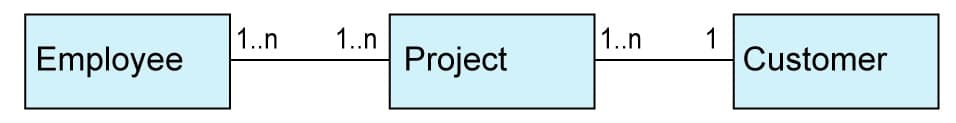
Assume that a group of employees in a particular team is working across different projects for different customers. The entity relationship diagram (ERD) given in Figure 1 gives an idea about the association between an employee, a project and a customer.

An employee could be working on one or more projects. A project could also have one or more employees. A project is targeted to be delivered to only one customer (in our example). A customer may be involved with multiple projects.

Note: Data about each of these entities could be modelled in a relational table of the same name. We will discuss more about tables in a subsequent section.

Now, the management may be interested in answers to different questions based on the data available, like how do we find out the summary effort spent by the team on a particular customer over a period of time? Or, what is the actual effort spent on a project till date (and how does it compare with the planned effort)?

To begin with, a part of the solution will have to be about deciding where and how to store the data. Here, we are first talking about the persistence layer for the information collected. While Python could be used to develop a full-fledged solution with a layer managing the data along with access to it (which could be made independent of the format in which data is stored), in this column, we will restrict ourselves to using Python to store and retrieve data in database tables (both in memory, and in a file or in a SQL server). In this way, we will focus more on the DB layer and on access, and less on concepts like exposing a suitable middleware layer which could handle the same.

A brief introduction to an RDBMS
The entity relationship model was introduced by Peter Chen. It provided a mathematical basis for analysis and modelling of entities and relationships in a problem or solution domain. The concept of a relational database management system (RDBMS) was developed by E.F. Codd. He proposed 12 rules that needed to be followed by a database to be called a relational database. Over time, the term has been reduced to the more common shorter form–database—tending to represent only the storage and retrieval part of the RDBMS.

So what is an RDBMS? In its essence, the idea is to model entities in a problem or solution domain into tables that capture the most essential data related to that entity, which helps us to identify and model its most important functionality and behaviour. While the entities themselves get represented by tables, the association between entities could also be represented by tables. So a database is made up of a collection of tables which together represent the data that one wants to collect and organise, with respect to the domain that is being modelled in the solution.

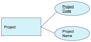
To make the idea of a table more concrete, let us go back to the entities that we wrote about in the previous section. Each entity, project, employee and customer could be represented by a corresponding table in the database. In its simplest form, a project could be made up of the following attributes—project name and project code or ID. We could represent them simply, as shown in Figure 2, with ‘Project Code’ being the primary key of this entity. A primary key serves to identify instances of the entity, uniquely, within the system to be worked with. ‘Project Name’ could also serve as an alternate key in this case, as long as a project name is not reused.

There could be many more optional attributes, depending upon what is needed in the system, like project start date, project cost planned, project manager, etc, which we are not including for now.

An employee works on one or more projects at any given time. The same association can be modelled as shown in Figure 3. The combination of keys shown in the figure uniquely identifies this association (employee name, project name, start date and end date), as the same employee may be assigned to different projects at different times.

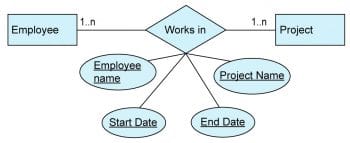
For the purpose of this column, let’s simplify such an association with the following attributes, as shown in the table below, to make it easier to show simple examples of data entry and retrieval for the summary data stated in the problem statement.

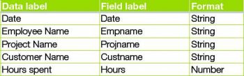
Note: The above table is neither optimised nor normalised. For the purposes of this column, however, this simplicity will be welcome.

A brief introduction to SQL
SQL or Structured Query Language is a specialised language used to work with RDBMSs. It has components that help define the structure of and create tables (CREATE statement), modify data in the tables (using INSERT, UPDATE, DELETE statements) and, most importantly, retrieve (SELECT) the data with syntax to filter records and manipulate results, as per needs. RDBMS systems are supposed to give a robust interface optimised for very fast data retrieval, even with a large number of records.

The SQL statement to create our table of interest, which we could call workdata, will look like what follows in SQLite3:

CREATE table workdata (date text, empname text, projname text, custname text, hours int)

To insert data records, let’s use the following INSERT SQL statement:

INSERT INTO workdata VALUES(‘01/01/2015’, ‘john’, ‘projectA’,’customerA’,8)

To query records for projectA, we could execute the following SELECT SQL statement:

SELECT * FROM workdata WHERE projname = ‘projectA’

To remove records for projectA, we could execute the following DELETE SQL statement:

DELETE FROM workdata WHERE projname = ‘projectA’

Note: If you omit the WHERE clause in the DELETE FROM statement, it will delete all records in the table.

An introduction to SQLite3 by creating and using a table with data
It is common to find an application, which works with data, to be designed with a data layer that works with a database system, most commonly an RDBMS. An industry level RDBMS, though, is a big beast to handle, with its own server and hardware requirements. A database server also requires some dedicated set-up and management expertise. Most applications, though, do not need such an extensive database system to work with. In the light of this, it is nice to note that Python comes with package SQLite3 with the default installation from Python 2.5. It conforms to a non-standard SQL version as specified in Python DB-API 2.0. The following is quoted verbatim from the SQLite3 documentation:

“SQLite is a C library that provides a lightweight disk-based database that doesn’t require a separate server process and allows accessing the database using a non-standard variant of the SQL query language. Some applications can use SQLite for internal data storage. It’s also possible to prototype an application using SQLite and then port the code to a larger database such as PostgreSQL or Oracle.”

Interfaces available with SQLite3
1. sqlite3.connect(dbname): The connect call creates a database connection to the database file specified by the dbname parameter and returns an object of type Connection. The dbname could also use the special value of “:memory:” to create an in-memory database, though the database ceases to exist once the connection is closed.
2. Connection.cursor(): This call helps create a Cursor object for the database connection. The Cursor object is the Python abstraction for creating multiple execution environments through the same database connection. cursors provide interfaces for SQL execution and parsing of results.
3. Cursor.execute(sql): This interface helps execute a single SQL statement as specified in the string parameter sql. There are other interfaces available to execute many SQL statements: executemany, as also ways to execute a script: executescript
4. Cursor.fetchone(): If preceded by a query execution, this interface returns a single sequence of the result set, as a tuple by default, or None object if no more results exist. So if you have multiple records returned from a query and would like to process them one by one, you would need to call this many times till a None record is returned. There are other interfaces like fetchmany(size) to fetch a list of records of a specified size. Also, fetchall() fetches all records in the same call, and returns a complete list of records from the query execution.
5. Connection.commit(): This interface commits the changes to the database. If there were DDL or DML statements executed, they need to be committed to the database for the changes to persist.
6. sqlite3.Row: This type can be used as a row_factory instance for the connection object. By default, the results of a query execution are handled as a tuple with indexed access to the attributes or values of the tuple. Using a row_factory, one can make custom access of the values using attribute names for mapping, which are lot more meaningful. While SQLite3 allows you to define your custom row_factory mapping, I strongly recommend that you use the built-in sqlite3.Row to access the results conveniently using column names.
Let us look at the above interfaces at work using the Python command line. In the first segment below, we connect to a test.db as a database file and open a cursor to the same connection.

>>> import sqlite3
>>> conn = sqlite3.connect(‘test.db’)
>>> c=conn.cursor()

We then create the table of interest and insert one record for projectA for employee john and commit the changes.

>>> c.execute(‘’’CREATE table workdata (date text, empname text, projname text,
custname text, hours int)
... ‘’’)
<sqlite3.Cursor object at 0x00000000021C1B20>
>>> c.execute(“INSERT INTO workdata VALUES(‘01/01/2015’, ‘john’, ‘projectA’,’cus
tomerA’,8)”)
<sqlite3.Cursor object at 0x00000000021C1B20>
>>> conn.commit()

We can then query for records of interest using a select query. We can see that the fetchone() call returns a record tuple, by default.

>>> c.execute(“SELECT * FROM workdata WHERE projname = ‘projectA’”)
<sqlite3.Cursor object at 0x00000000021C1B20>
>>> c.fetchone()
(u’01/01/2015’, u’john’, u’projectA’, u’customerA’, 8)

By default, we can access the data returned in a tuple by index based access. For example, in the code segment below, row variable with default factory binding, allows access to the different attributes by index offset. This requires us to hard code the index offset to map to a particular column name. And this would need to be changed if the position of the column changes.

>>> row = c.fetchone()
>>> print row[0]
01/01/2015
>>> print row[1]
john
>>> print row[2]
projectA
>>> print row[3]
customerA

By using sqlite3.Row binding we can access the same data in a more natural way using name binding. We can use the column name as the key to access the value fetched in the query, as shown in the following segment.

>>> import sqlite3
>>> conn = sqlite3.connect(‘test.db’)
>>> conn.row_factory = sqlite3.Row
>>> c = conn.cursor()
...
>>> c.execute(“SELECT * FROM workdata WHERE projname = ‘projectA’”)
<sqlite3.Cursor object at 0x000000000221EB20>
>>> row = c.fetchone()
>>> type(row)
<type ‘sqlite3.Row’>
>>> print row[“empname”]
john

We can see above that the type of record returned now is sqlite3.Row and this gives us access using the column name to retrieve the value. Before we do that though, let us insert the following values into the table using an executemany() function. This is an easy way to execute multiple SQLs in one statement.

>>> records = [(‘01/01/2015’,’miller’,’projectA’,’customerA’,8),
... (‘01/01/2015’,’john’,’projectA’,’customerA’,8),
... (‘02/01/2015’,’john’,’projectA’,’customerA’,8),
... (‘02/01/2015’,’miller’,’projectB’,’customerB’,8)]
>>> c.executemany(‘INSERT into workdata VALUES(?,?,?,?,?)’,records)
<sqlite3.Cursor object at 0x000000000224EB20>
>>> conn.commit()

Note: The recommended way for parameter substitution is using the “?” placeholder for parameters. Using Python string formatting methods leads to undesirable security vulnerabilities, like code injection through an SQL injection attack.

Now, using sqlite3.Row binding, one can write code to access data based on column name, for example, to sum up the hours spent on ‘projectA’, like in the code segment below.

>>> for row in c.execute(“SELECT * FROM workdata WHERE projname = ‘projectA’”):
...     projectAhours+=row[‘hours’]
...
>>> print “Time spent on ProjectA :” + repr(projectAhours) + “ hours”
Time spent on ProjectA :24 hours

An alternate way of using the power of the SQL summation function is illustrated in the following code, which could be faster as the summary is being done in the database layer itself.

>>> c.execute(“SELECT SUM(hours) as totalhours FROM workdata where projname=’pro
jectA’”)
<sqlite3.Cursor object at 0x00000000021EEB20>
>>> sumrow=c.fetchone()
>>> print “Time spent on ProjectA :” + repr(sumrow[‘totalhours’]) + “ hours”
Time spent on ProjectA :24 hours

Note: The repr method used above to make int a printable string is similar in functionality to the str method, with one difference—repr gives an official representation while str gives an informal representation. For example, repr prints strings with quotes in the output, while str does not.

Working with a MySQL database to connect and run the same program
Having worked with SQLite3, now is a good time to move to MySQL, which vies for the title ‘The world’s most popular open source database’. In the current section, I assume that you have installed the MySQL database. For the purpose of this column, I have installed MySQL community edition (5.6.24 MySQL Community Server (GPL)). Also, for the sake of simplicity, I will be showing MySQL connections running out of localhost only. I leave it to you to check out more advanced uses of MySQL.
Since MySQLdb also conforms to the Python DB API 2.0 standard, there are very few changes needed to get our code to work with MySQL. To start with, since MySQL is a full fledged RDBMS, the call to make a connection object is more detailed in comparison to the file based SQLite3. We need to specify the server name (which would be localhost when the client runs on the same machine), the user name and password for the account with which we want to access the database, and last of all, the database itself to which we want to connect.

>>> import MySQLdb
>>> conn = MySQLdb.connect(host=”localhost”, user=”uname”, passwd=”pwd”,db=”test“)

Since the cursor object remains the same, the rest of the previous code continues to work well here too, with MySQLdb.

>>> c = conn.cursor()
>>> c.execute(‘’’CREATE table workdata (date text, empname text, projname text,c
ustname text, hours int)’’’)
0L
>>> conn.commit()
>>> c.execute(“INSERT INTO workdata VALUES(‘01/01/2015’, ‘john’, ‘projectA’,’cus
tomerA’,8)”)
1L
>>> conn.commit()

Further, to do name binding to the row output of the SELECT SQL with SQLite3 we used sqlite3.Row for the row_factory. With MySQLdb we need to use a different method to do name binding for the result set. We have a specific cursor type defined to be able to access the results as a dictionary object. When we create the cursor object, we need to pass and select the type as MySQLdb.cursors.DictCursor.

>>> dc = conn.cursor(MySQLdb.cursors.DictCursor)
>>> dc.execute(“SELECT * FROM workdata WHERE projname = ‘projectA’”)
1L
>>> row=dc.fetchone()
>>> type(row)
<type ‘dict’>
>>> row[‘empname’]
‘john’

Note: 1. The execute() call returns the number of records affected; we would see later that executemany() too does the same.
2. The type of row object returned by fetchone() is ‘dict’.

The next difference comes at the executemany() function. While the SQLite3 version accepted parameter substitution with ? as placeholder, the MySQLdb version accepts only %s as shown below:

>>> workrecords = [(‘01/01/2015’,’miller’,’projectA’,’customerA’,8),
... (‘01/01/2015’,’john’,’projectA’,’customerA’,8),
... (‘02/01/2015’,’john’,’projectA’,’customerA’,8),
... (‘02/01/2015’,’miller’,’projectB’,’customerB’,8)]
>>> c.executemany(‘INSERT into workdata VALUES(%s,%s,%s,%s,%s)’,workrecords)
4L
>>> conn.commit()

Another difference is in the way we access the results of the query execution. With SQLite3, we could directly iterate over the results of the execute call and do operations with the data retrieved. Instead, with the dict cursor, we will have to iterate over the fetchall() call.

>>> projectAhours=0
>>> c.execute(“SELECT * FROM workdata WHERE projname = ‘projectA’”)
3L
>>> for row in c.fetchall():
...     projectAhours+=row[‘hours’]
...
>>> print “Time spent on ProjectA :”+repr(projectAhours)+ “ hours”
Time spent on ProjectA :24L hours
>>> print “Time spent on ProjectA :”+str(projectAhours)+ “ hours”
Time spent on ProjectA :24 hours

Note: The repr() call returns a value with an L suffix to indicate it to be long, while the str() call returns only the number.

Finally, the query summary function result is also visible below. The difference here is only with respect to how the repr() function works, while str() remains a better choice.

>>> c.execute(“SELECT SUM(hours) as totalhours FROM workdata where projname=’pro
jectA’”)
1L
>>> sumrow=c.fetchone()
>>> print “Time spent on ProjectA :” + repr(sumrow[‘totalhours’]) + “ hours”
Time spent on ProjectA :Decimal(‘24’) hours
>>> print “Time spent on ProjectA :” + str(sumrow[‘totalhours’]) + “ hours”
Time spent on ProjectA :24 hours

Using object relational DBMSs to avoid writing SQL queries
ORM (object relational mapping) packages allow the user to create and access data in tables without writing SQL statements. A package that we will explore in this article is peewee, and we will look at some of its uses to get the work done using MySQL.
peewee provides the MySQLDatabase interface to create a connection to a MySQL database. As usual, it takes the database name as the first argument, and then the user name and password to make the connection.

>>> import peewee
>>> from peewee import *
>>> mysql_db = MySQLDatabase(‘test’, user=’user’, passwd = ‘pwd’)

By deriving from the peewee.Model we can create the structure of the table that we desire and model it as a class. Instances of this can be saved as new records, and the class itself can act as the ORM mapper to provide other functionalities of filtering and querying, as shown below.

>>> class NewWorkData(peewee.Model):
...     date = peewee.CharField()
...     empname = peewee.CharField()
...     projname = peewee.CharField()
...     custname = peewee.CharField()
...     hours = peewee.IntegerField()
...
...     class Meta:
...             database = mysql_db
...
>>> NewWorkData.create_table()
>>> todaysdata = NewWorkData(date=’11/05/15’,empname=’john’,projname=’projectA’,
custname=’customerA’,hours = 8)
>>> todaysdata.save()
1
>>> for data in NewWorkData.filter(projname=’projectA’):
...     print data.hours
...
8