 Since the last decade, the R programming language has assumed importance as the most important tool for computational statistics, visualisation and data science. R is being used more and more to solve the most complex problems in computational biology, actuarial science and quantitative marketing.
Since data volumes are increasing exponentially, storage has become increasingly complex. Rudimentary tips and techniques have become obsolete and no longer result in improved efficiency. Currently, complex statistical and probabilistic approaches have become the de facto standard for major IT companies to harness deep insights from Big Data. In this context, R is one of the best environments for mathematical and graphical analysis on data sets. Major IT players like IBM, SAS, Statsoft, etc, are increasingly integrating R into their products.
R code: A walk through
Numerical computation: It is very easy to use R for basic analytical tasks. The following code creates a sample data of claims made in the year 2013 and subsequent claims that turned out to be fraudulent for a hypothetical insurance company ABC Insurance Inc. Then, the code performs some simple commonly used statistical tasks like calculating extended mean (number of values greater than 29 upon total number of values), standard deviation, degree of correlation, etc. Finally, the last statement performs a test to check whether the means of two input variables are equal. A null hypothesis results if the means are equal; else, an alternative hypothesis emerges. The p-value in the result shows off the probability of obtaining a test (here, it is extremely small as there is a huge difference between the means):
> claim_2013 <- c(30,20,40,12,13,17,28,33,27,22,31,16);
> fraud_2013 <- c(8,4,11,3,1,2,11,17,12,10,8,7);
> summary(claim_2013);
> mean(claim_2013>29);
Output: [1] 0.3333333
> sd(claim_2013);
Output: [1] 8.764166
> cor(claim_2013,fraud_2013);
Output: [1] 0.7729799
> table(fraud_2013,claim_2013);
> t.test(claim_2013,fraud_2013);
<strong>Probabilistic distribution: </strong>R provides an over-abundance of probabilistic function support. It is the scenario that decides the domain of probabilistic applicability.
<strong>Exponential distribution:</strong> This is an estimator of the occurrence of an event in a given time frame, where all other events are independent and occur at a constant rate. Assume that a project’s stub processing rate is ? = 1/5 per sec. Then, the probability that the stub is completed in less than two seconds is:
>pexp(2, rate=1/5);
<a style="text-align: center; font-family: Georgia, 'Times New Roman', 'Bitstream Charter', Times, serif; font-size: 14px; line-height: 1.5em;" href="https://www.opensourceforu.com/wp-content/uploads/2014/10/Figure-1-Poisson.jpg"><img class="size-medium wp-image-13975" alt="Figure 1 Poisson" src="https://www.opensourceforu.com/wp-content/uploads/2014/10/Figure-1-Poisson-350x187.jpg" width="350" height="187" /></a>
- Figure 1 Poisson
<strong>Binomial distribution:</strong> This is an estimator of the exact probability of an occurrence. If the probability of a program failing is 0.3, then the following code computes the probability of three failures in an observation of 10 instances:
>dbinom(3, size=10, prob=0.3);
>pbinom(3, size=10, prob=0.3);
The second statement computes the probability of three or less failures.
<strong>Gaussian distribution:</strong> This is the probability stating that an outcome will fall between two pre-calculated values. If the fraud data given above follows normal distribution, the following code computes the probability that the fraud cases in a month are less than 10:
>m <- mean(fraud_2013);
>s <- sd(fraud_2013);
> pnorm(9, mean=m, sd=s);
<strong>Graphical data analysis
Probabilistic plots:</strong> These are often needed to check and demonstrate fluctuating data values over some fixed range, like time. dnorm, pnorm, qnorm and rnorm are a few basic normal distributions that provide density, the distribution function, quantile function and random deviation, respectively, over the input mean and standard deviation. Let us generate some random number and check its probability density function. Such random generations are often used to train neural nets:
>ndata <- rnorm(100);
>ndata <- sort(ndata);
>hist(ndata,probability=TRUE);
>lines(density(ndata),col=“blue”);
>d <- dnorm(ndata);
>lines(ndata,d,col=“red”);
The Poisson distribution (<em><a href="http://mathworld.wolfram.com/PoissonDistribution.html" target="_blank">http://mathworld.wolfram.com/<wbr />PoissonDistribution.html</a>)</em> is used to get outcomes when the average successful outcome over a specified region is known. For the hypothetical insurance company, the average fraudulent claims related to the property and casualty sector in the first quarter of the year are given. Using the Poisson distribution, we can hypothesise the exact number of fraud claims. Figure 1 graphically plots the distribution for the exact number (0 to 10) of fraudulent claims with different means (1 to 6). From the figure, it is clear that as the rate increases, the high number of fraud claims also shift towards the right of the x axis.
par(mfrow=c(2,3))
avg <- 1:6
x <- 0:10
for(i in avg){
pvar <- dpois(x, avg[i])
barplot(pvar,names.arg=c("0", "1", "2", "3", "4",
"5", "6", "7", "8", "9", "10"),ylab=expression(P(x)),
ylim=c(0,.4), col=“red”)
title(main = substitute(Rate == i,list(i=i)))
} //Poisson.png
In the field of data analytics, we are often concerned with the coherency in data. One common way to ensure this is regression testing. It is a type of curve fitting (in case of multiple regressions) and checks the intercepts made at different instances of a fixed variable. Such techniques are widely used to check and select the convergence of data from the collections of random data. Regressions of a higher degree (two or more) produce a more accurate fitting, but if such a curve fitting produces a NaN error (not a number), just ignore those data points.
>attach(cars);
>lm(speed~dist);
>claim_2013 <- c(30,20,40,12,13,17,28,33,27,22,31,16);
>fraud_2013 <- c(8,4,11,3,1,2,11,17,12,10,8,7);
>plot(claim_2013,fraud_2013);
>poly2 <- lm(fraud_2013 ~ poly(claim_2013, 2, raw=TRUE));
>poly3 <- lm(fraud_2013 ~ poly(claim_2013, 3, raw=TRUE));
>summary(poly2);
>summary(poly3);
>plot(poly2);
>plot(poly3);
<strong>Interactive plots:</strong> One widely used package for interactive plotting is iplots. Use install.packages(“iplots”); to install iplot and library(“iplots”); to load it in R. There are plenty of sample data sets in R that can be used for demonstration and learning purposes. You can issue the command data(); at the R prompt to check the list of available datasets. To check the datasets available across different packages, run data(package = .packages(all.available = TRUE));. We can then install the respective package with the install command and the associated dataset will be available to us. For reference, some datasets are available in csv/doc format at <em><a href="http://vincentarelbundock.github.io/Rdatasets/datasets.html" target="_blank">http://vincentarelbundock.<wbr />github.io/Rdatasets/datasets.<wbr />html</a>. </em>

<em> </em>
>ihist(uspop);
>imosaic(cars);
>ipcp(mtcars);

Another package worth mentioning for interactive plots is ggplot2. Install and load it as mentioned above. It is capable of handling multilayer graphics quite efficiently with plenty of options to delineate details in graphs. More information on ggplot can be obtained at its home site <em><a href="http://ggplot2.org/" target="_blank">http://ggplot2.org/</a>.</em> The following code presents some tweaks of ggplot:
> qplot(data=cars,x=speed);
> qplot(data=mpg,x=displ,y=hwy,color=manufacturer);
> qplot(data=cars,x=speed,y=dist,color=dist,facets = ~dist);
>qplot(displ, hwy, data=mpg, geom=c("point", "smooth"),method="lm",color=manufacturer); //ggplot.png

<strong>Working on data in R</strong>
<strong>CSV</strong>: Business analysts and testing engineers use R directly over the CSV/Excel file to analyse or summarise data statistically or graphically; such data are usually not generated in real time. A simple read command, with the header attribute as true, directs R to load data for manipulation in the CSV format. The following snippet reads data from a CSV file and writes the same data by creating another CSV file:
>x = read.csv("e:/Incident_Jan.csv", header = TRUE);
>write.table(x,file = "e:/Incident_Jan_dump.csv", sep = ",",col.names = NA);

<strong>Connecting R to the data source (MySQL):</strong>  With Big Data in action, real time access to the data source becomes a necessity. Though CSV/Excel serve the purpose of data manipulation and summarisation, real analytics is achieved only when mathematical models are readily integrated with a live data source. There are two ways to connect R to a data source like MySQL. Any Java developer would be well aware of JDBC; in R, we use RJDBC to create a data source connection. Before proceeding, we must install the RJDBC package in an R environment. This package uses the same jar that is used to connect Java code to the MySQl database.
>install.packages("RJDBC");
>library(RJDBC);
>PATH <- “Replace with path of mysql-connector-java-5.0.8-bin.jar”
>drv <- JDBC("com.mysql.jdbc.Driver",PATH);
>conn <- dbConnect(drv,"jdbc:mysql://SERVER_NAME/claim","username","xxxx")
>res <- dbGetQuery(conn,"select * from rcode");

The first snippet installs RJDBC in the R environment; alternatively, we can use a GUI by going to the Packages tab from the menu, selecting ‘<em>Install Packages</em>’ and clicking on RJDBC. The second snippet loads the installed RJDBC package into the environment; third, we create a path variable containing the Java MySQL connector jar file. In the fourth statement, to connect a database named ‘<em>claim</em>’, replace ‘<em>SERVER_NAME</em>’ with the name of your server, ‘<em>username</em>’ with your MySQL username, and ‘<em>xxxx</em>’ with your MySQL password. From here on, we are connected to the database ‘<em>claim</em>’, and can run any SQL query for all the tables inside this database using the method dbGetQuery, which takes the connection object and SQL query as arguments. Once all this is done, we can use any R mathematical model or graphical analyser on the retrieved query. As an example, to graphically plot the whole table, run - plot(res); to summarise the table for the retrieved tuples, run - summary(res); to check the correlation between retrieved attributes, run - cor(res); etc. This allows a researcher direct access to the data without having to first export it from a database and then import it from a CSV file or enter it directly into R.
Another technique to connect MySQL is by using RMySQL—a native driver to provide a database interface for R. To know more about the driver, refer to <a href="http://cran.r-project.org/web/packages/RMySQL/RMySQL.pdf" target="_blank">http://cran.r-project.org/web/<wbr />packages/RMySQL/RMySQL.pdf</a>.

<strong>Rendering R as XML (portable data format):</strong> With the increasing prevalence of Service Orientation Architecture (SOA) and cloud services like SaaS and Paas, we are very often interested in exposing our results via common information sharing platforms like XML or Jason. R provides an XML package to do all the tricks and tradeoffs with XML. The following snippet describes XML loading and summarisation:<em></em>
>install.packages("XML");
>library(XML);
>dat <- xmlParse("URL")
> xmlToDataFrame(getNodeSet(dat, "//value"));

Use the actual URL of the XML file in place of ‘URL’ in the third statement. The next statement lists compatible data in row/column order. The node name is listed as the header of the respective column while its values are listed in rows.
A more reasonable approach in R is exposing results as XML. The following scenario does exactly this. Let there be two instances of probability distribution, namely, the current and the previous one for two probability distribution functions —Poisson and Exponential. The code follows below:
>x1<-ppois(16, lambda=12);
>x2<- pexp(2, rate=1/3);
>y1<-ppois(16, lambda=10);
>y2<- pexp(2, rate=1/2);
>xn <- xmlTree("probability_distribution");
>xn$addTag("cur_val",close="F");
>xn$addTag("poisson",x1);
>xn$addTag("exponential",x2);
>xn$closeTag();
>xn$addTag("prev_val",close="F");
>xn$addTag("poisson",y1);
>xn$addTag("exponential",y2);
>xn$closeTag();
>xn$value();

Let’s begin by creating a root node for the XML document. Then we go forward by creating child nodes using the method addtag (addtag maintains parent child tree structure of XML). Once finished with adding tags, the value preceded by the root node name displays the XML document in a tree structure.

<strong>Advance data analytics</strong>
<strong>Neural networks (facilitating machine learning):</strong> Before proceeding further, we need to power up our R environment for neural network support by executing the following command at the R prompt install.packages("neuralnet"); and load using command library (neuralnet); into the R environment. Neural networks are complex mathematical frameworks that often contain mapping of sigmoid with the inverse sigmoid function, and have sine and cosine in an overlapped state to provide timeliness in computation. To provide learning capabilities, the resultant equation is differentiated and integrated several times over different parameters depending on the scenario. (A differentiating parameter in the case of banking could be the maximum purchases made by an individual over a certain period—for example, more electronic goods purchased during Diwali than at any other time in the year.) In short, it may take a while to get the result after running a neural net. Later, we will discuss combinatorial explosion, a common phenomenon related to neurons.
For a simple use case scenario, let’s make a neural network to learn about a company’s profit data at 60 instances; then we direct it to predict the next instance, i.e., the 61st.
>t1 <-  as.data.frame(1:60);
>t2 <-  2*t1 - 1;
>trainingdata <- cbind(t1,t2);
> colnames(trainingdata) <- c("Input","Output");
> net.series <- neuralnet(Output~Input,trainingdata, hidden=20, threshold=0.01);
> plot(net.series);
> net.results <- compute(net.series, 61);

In the above code, Statement 1 loads numeral 1 to 60 into t1, followed by loading of data into t2 where each instance = 2*t1-1. The third statement creates a training data set for the neural network, binding together the numerals with its instance, i.e., t2 with t1. Next, let’s term t1 as input and t2 as output to make the neural network understand what is input into it and what it should learn. In Statement 5, actual learning takes place with 20 hidden neurons (the greater the number, the greater is the efficiency or lesser the approximation); .01 is the threshold value where the neuron activates itself for input. In Statement 6, we see a graphical plot of this learning, labelled by weights (+ and -). Refer to Figure 3. Now the neural network is ready to predict the 61st instance for us, and Statement 7 does exactly that. The deviation from the actual result is due to very few instances to train neurons. As the learning instance increases, the result will converge more accurately. A good read on training neural nets is provided in the following research journal: <a href="http://journal.r-project.org/archive/2010-1/RJournal_2010-1_Guenther+Fritsch.pdf" target="_blank">http://journal.r-project.org/<wbr />archive/2010-1/RJournal_2010-<wbr />1_Guenther+Fritsch.pdf</a>
Genetic algorithms (GA): This is the class of algorithms that can leverage evolution-based heuristic techniques to solve a problem. GA is represented by a chromosome like data structure, which uses recursive recombination or search techniques. GA is applied over the problem domain in which the outcome is very unpredictable and the process of generating the outcome contains complex inter-related modules. For example, in the case of AIDS, the human immunodeficiency virus becomes resistant to antibiotics after a definite span of time, after which the patient is dosed with a completely new kind of antibiotic. This new antibiotic is prepared by analysing the pattern of the human immunodeficiency virus and its resilient nature. As time passes, finding the required pattern becomes very complex and, hence, leads to inaccuracy. The GA, with its evolutionary-based theory, is a boon in this field. The genes defined by the algorithm generate an evolutionary-based antibiotic for the respective patient. One such case to be mentioned here is IBM’s EuResist genomics project in Africa.
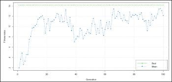
The following code begins by installing and loading the GA package into the R environment. We then define a function which will be used for fitting; it contains a summation of the extended sigmoid function and sine function. The fifth statement performs the necessary fitting within maximum and minimum limits. We can then summarise the result and can check its behaviour by plotting it.
>install.packages(“GA”);
>library(“GA”);
>f <- function(x){ 1/(exp(x)+exp(-x)) + x*sin(x) };
>plot(f,-15,15);
>geneticAl <- ga(type = "real-valued", fitness = f, min = -15, max = 15);
>summary(geneticAl);
>plot(geneticAl); //

Refer to Figure 4

<strong>A trade off (paradox of exponential degradation):</strong> The type of problem where the algorithms defined run in super polynomial time [O(2n) or O(nn)] rather than polynomial time [O(nk) for some constant k] are called combinatorial explosion problems or non polynomial. Neural networks and genetic algorithms often fall into the category of non polynomial. Neural networks contain neurons that are complex mathematical models; several thousands of neurons are contained in a single neural net and any practical learning network comprises several hundreds of neural nets, taking the mathematical equations to a very high degree. The higher the degree, the greater is the efficiency. But the higher degree has an adverse effect on computability time (ignoring space complexity). The idea of limiting and approximating results is called amortized analysis. R code does not provide any inbuilt tools to check combinatorial explosion.


