Using Scilab with the McCabe-Thiele Method

Cross-platform, open source numerical computational package, Scilab, can be used for image enhancement, fluid dynamics simulations and numerical optimisation, among other things. When used with the McCabe-Thiele method, which is said to be the simplest and perhaps most instructive method for the analysis of binary distillation, the combination is formidable.

The McCabe-Thiele method was published 90 years ago by Warren L. McCabe and Ernest W. Thiele in an article titled ‘Graphical Design of Fractionating Columns’. To use their own words, “…the method consists essentially in drawing, on the same rectangular plot, the equilibrium curve for vapour and liquid compositions and straight lines representing the equations for enrichment from plate to plate, and passing from one to another in a series of steps.” Scilab is an open source software for numerical computation with a syntax similar to MathWorks’ MATLAB. The aim of this article is to show how Scilab can be used to plot the McCabe-Thiele diagram and simulate the distillation of a binary mixture. All the Scilab examples presented here are made under Linux Mint 17 Xfce.

The vapour-liquid equilibrium curve
First, it’s necessary to plot the vapour-liquid equilibrium (VLE) curve for the most volatile (lower-boiling) component in the mixture. For the two mixtures discussed here (ethanol/water and chloroform/methanol), the data points (x,y) are taken from the third reference given at the end of this article. Note that the point at which the VLE curve cuts the diagram on the diagonal is called the azeotrope. At this point, the vapour phase has the same composition as the liquid phase and the mixture cannot be separated by a simple distillation. The data points are now fitted with three different techniques to obtain the VLE curve equation:

• Cubic spline monotone
• Rational function 1 (with four coefficients)
• Rational function 2 (with six coefficients)

// Rational function 1
deff(“[y]=f(a,b,c,d,x)”,”y=((a+b*x)./(1+c*x+d*x.^2))”);
deff(“[e]=res(A,x,y)”,”e=f(A(1),A(2),A(3),A(4),x)-y”);
Ainit=[1;1;1;1];
[S,coe]=leastsq(list(res,x,y),Ainit);
yp1=f(coe(1),coe(2),coe(3),coe(4),xx);

// Rational function 2
deff(“[y]=f(a,b,c,d,e,f,x)”,”y=((a+b*x+c*x.^2)./(1+d*x+e*x.^2+f*x.^3))”); deff(“[e]=res(A,x,y)”,”e=f(A(1),A(2), A(3),A(4),A(5),A(6),x)-y”);
Ainit=[1;1;1;1;1;1];
[S,coe]=leastsq(list(res,x,y),Ainit);
yp2=f(coe(1),coe(2),coe(3),coe(4),coe(5),coe(6),xx);

// Cubic spline monotone
df=splin(x,y,”monotone”);
[yyf,yy1f,yy2f]=interp(xx,x,y,df);

plot([0,1],[0,1],”c-”,.. // Diagonal
xx,yp1,”b-.”,.. // Rational function 1
xx,yp2,”g-”,.. // Rational function 2
xx,yyf,”k-.”,.. // Cubic spline monotone
x,y,”ko”); // Data points

The Rational function 2 was chosen as the most interesting (see the green curve in Figures 1 and 2) and six coefficients will be used to define each VLE curve. A simple polynomial model was not chosen because of its instability.

The McCabe-Thiele method
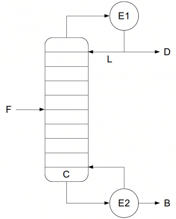
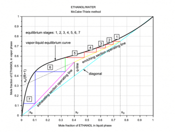
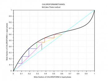
The next step is to draw the q-line. This line starts on the diagonal at the xF value and has a slope which depends on the feed thermal conditions. In Figures 4 and 5, because we have a saturated-liquid feed, the q-line is vertical. For the other q-line types, see the third and fourth references at the end of this article. Then it’s possible to draw another line called the operating line for the enriching section (the section above the feed inlet, the yellow line in Figures 4 and 5). This second line starts on the diagonal at the xD value and cuts the y-axis at the value xD/(R+1). The last line is called the operating line for the exhausting section (the section below the feed inlet, the magenta line in Figures 4 and 5). This third line starts on the diagonal at the xB value and ends at the intersection (xi,yi) of the two previous lines.

xF=0.35; // Feed mole fraction
xD=0.6; // Distillate mole fraction
xB=0.05; // Bottom product mole fraction
R=1.5; // Reflux ratio R=L/D
q=1; // Feed thermal conditions
xi=(-(q-1)*(1-R/(R+1))*xD-xF)/((q-1)*R/(R+1)-q); // Intersection x point
yi=(xF+xD*q/R)/(1+q/R); // Intersection y point
plot([0,1],[0,1],”c-”,.. // Diagonal
xx,yp,”k-”,.. // Rational function 2
[xF,xi],[xF,yi],”k-”,.. // q-line
[xD,xi],[xD,yi],”y-”,.. // Operating line enriching section
[xB,xi],[xB,yi],”m-”); // Operating line exhausting section

Finally, it’s possible to draw the steps between the operating lines and the VLE curve and then count them (Figures 4 and 5). These steps represent the equilibrium stages (theoretical plates) required to carry out the distillation at the given conditions. The required number of theoretical plates is seven for the example in Figure 4, and six for the example in Figure 5. The Scilab code used to plot the operating lines and the equilibrium stages is adapted to Scilab from the MATLAB code written by Housam Binous, as reported in the fifth reference at the end of this article.

// VLE curve equation
function f=equilib(x)
f=y-((coe(1)+coe(2)*x+coe(3)*x.^2)./(1+coe(4)*x+coe(5)*x.^2+coe(6)*x.^3));
endfunction

// Enriching section
i=1;
xp(1)=xD;
yp(1)=xD;
y=xD;
while (xp(i)>xi),
xp(i+1)=fsolve(0.01,equilib); // Steps x coordinates
yp(i+1)=R/(R+1)*xp(i+1)+xD/(R+1); // Steps y coordinates
y=yp(i+1);
plot([xp(i),xp(i+1)],[yp(i),yp(i)],”r-”); // Steps plot
if (xp(i+1)>xi) then
plot([xp(i+1),xp(i+1)],[yp(i),yp(i+1)],”r-”); // Vertical lines
end
i=i+1;
end

// Exhausting section
SS=(yi-xB)/(xi-xB);
yp(i)=SS*(xp(i)-xB)+xB;
y=yp(i);
plot([xp(i),xp(i)],[yp(i-1),yp(i)],”g-”); // Vertical line
while (xp(i)>xB),
xp(i+1)=fsolve(0.01,equilib); // Steps x coordinates
yp(i+1)=SS*(xp(i+1)-xB)+xB; // Steps y coordinates
y=yp(i+1);
plot([xp(i),xp(i+1)],[yp(i),yp(i)],”b-”); // Steps plot
if (xp(i+1)>xB) then
plot([xp(i+1),xp(i+1)],[yp(i),yp(i+1)],”b-”); // Vertical lines
end
i=i+1;
end
<a href="https://www.opensourceforu.com/?attachment_id=18091" rel="attachment wp-att-18091"><img class="alignnone size-medium wp-image-18091" src="https://www.opensourceforu.com/wp-content/uploads/2015/10/Untitled4-350x227.jpg" alt="Untitled" width="350" height="227" /></a>

With Scilab, it’s possible to calculate the equation of a vapour-liquid equilibrium curve with the use of a rational function, at least as a first guess. Probably, in the future, it will be necessary to improve this kind of rational function. Then it will be possible to simulate a distillation process to obtain the number of equilibrium stages. I hope this article will stimulate the reader’s curiosity about Scilab.

References
[1] McCabe, Thiele, Graphical Design of Fractionating Columns, Industrial and Engineering Chemistry, 1925, 17 (6), 605-611
[2] http://www.scilab.org, last visited on 26/12/2014
[3] Perry, Green, Maloney (editors), Perry’s Chemical Engineers Handbook, 7th edition, McGraw-Hill, New York, 1997
[4] Foust, Wenzel, Clump, Maus, Andersen, I principi delle operazioni unitarie (Principles of Unit Operations), Casa Editrice Ambrosiana, Milan, 1967
[5] http://www.mathworks.com/matlabcentral/fileexchange/ 4472-mccabe-thiele-method-for-an-ideal-binary-mixture, last visited on 26/12/2014.