


For the past three months, we have been trying to master ns-3. We had our tryst with socket programming, grasped the basics of Waf, Mercurial, Doxygen, etc, and finally we ran our first ns-3 script. But our aim is not to just run ns-3 scripts; we are in hot pursuit of data which, when processed, will yield information that might even change the history of computer networks. Thus, the ultimate aim of any simulation is to obtain data and information. There is a large amount of data available from an ns-3 script, which might even lead to information overload. As mentioned earlier, there are three different ways to harness this data from an ns-3 simulation. The log data, the trace file data and the topology animation. Of the three methods, the log data provides the least amount of information and we have covered it already. What matters now are the other two methods the trace files and topology animation. The topology animation is important because it confirms the topology visually, and trace analysis is important because thats where all our data lies.
I just want to mention the relative importance of animation and trace analysis. In one of my previous incarnations (when I was helping students with their ns-2 projects), I found them mostly worried about the animation and not about the trace file. I have also come across academicians who pester their students with the animation part of the simulation and not the trace file which actually is a treasure trove of information. But from experience, let me tell you something the animation part of the simulation in ns-2 or ns-3 is not your priority. It might be entertaining to view the animation of your topology but the real purpose of it is to confirm the topology and nothing more. So our priority is the trace file and its analysis, but due to popular demand, I will first discuss the setting up of NetAnim and running topology animations.
Installing NetAnim
Last time when we tried to run NetAnim, we discovered that NetAnim was not yet installed in our system. The QT4 development package is required to install NetAnim. If you do not have Internet connectivity in your system then please install the QT4 development package with installation files downloaded from elsewhere. If you are following the installation instructions given here, it is mandatory to have Internet connectivity in your system. If your operating system is Debian or Ubuntu, then execute the following commands in a terminal:
apt-get install mercurial
apt-get install qt4-dev-tools
If your operating system is Fedora, then type the following commands in the terminal:
yum install mercurial
yum install qt4
yum install qt4-devel
The above commands will take care of the QT4 development package installation. Now it is time to install NetAnim. If you have followed the installation instructions provided in the previous parts of this series, then you will have a directory named ns/ns-allinone-3.22/netanim-3.105. Open a terminal in this directory and execute the following command:
make clean
qmake NetAnim.pro
make
The command qmake NetAnim.pro might give you the following error message qmake: command not found. The utility called qmake automates the generation of Makefiles. qmake is not supported in some systems, in which case, execute the command qmake-qt4 NetAnim.pro instead of qmake NetAnim.pro and then execute the command make. This will finish the installation of NetAnim in your system, and you can see the ELF file (executable file format in Linux similar to an exe file in Windows) of NetAnim in the directory ns/ns-allinone-3.22/netanim-3.105. Now, you can run an instance of NetAnim by executing the command ./NetAnim in a terminal opened in this directory. But we still dont have an XML based animation trace file which will be used by NetAnim to show us the topology animation. So it is time to go through another ns-3 script, which will give us the XML file to feed NetAnim.
The script for animation and tracing
The ns-3 script named netanim1.cc given below will generate an animation trace file with the extension .xml and an ASCII trace file with extension .tr. You can download the file netanim1.cc and all the other script files discussed in this article from opensourceforu.com/article_source_code/august2015/ns3.zip. Running the ns-3 script is similar to what we did before with just the names changed.
#include <iostream>
#include ns3/core-module.h
#include ns3/network-module.h
#include ns3/internet-module.h
#include ns3/point-to-point-module.h
#include ns3/netanim-module.h
#include ns3/applications-module.h
#include ns3/point-to-point-layout-module.h
using namespace ns3;
using namespace std;
int main(int argc, char *argv[])
{
Config::SetDefault(ns3::OnOffApplication::PacketSize, UintegerValue (1024));
Config::SetDefault(ns3::OnOffApplication::DataRate, StringValue (100kb/s));
std::string animFile = netanim1.xml;
PointToPointHelper pointToPointRouter;
pointToPointRouter.SetDeviceAttribute(DataRate, StringValue(10Mbps));
pointToPointRouter.SetChannelAttribute(Delay, StringValue(1ms));
PointToPointHelper pointToPointEndNode;
pointToPointEndNode.SetDeviceAttribute(DataRate, StringValue(10Mbps));
pointToPointEndNode.SetChannelAttribute(Delay, StringValue(1ms));
PointToPointDumbbellHelper d(1, pointToPointEndNode, 1, pointToPointEndNode,
pointToPointRouter);
InternetStackHelper stack;
d.InstallStack (stack);
d.AssignIpv4Addresses(Ipv4AddressHelper(192.168.100.0, 255.255.255.0),
Ipv4AddressHelper(192.169.100.0, 255.255.255.0),
Ipv4AddressHelper(192.170.100.0, 255.255.255.0));
OnOffHelper clientHelper(ns3::UdpSocketFactory, Address());
clientHelper.SetAttribute(OnTime,StringValue(ns3::UniformRandomVariable));
clientHelper.SetAttribute(OffTime,StringValue(ns3::UniformRandomVariable));
ApplicationContainer clientApps;
AddressValue remoteAddress(InetSocketAddress(d.GetLeftIpv4Address(0), 5000));
clientHelper.SetAttribute(Remote, remoteAddress);
clientApps.Add(clientHelper.Install(d.GetRight(0)));
clientApps.Start(Seconds(1.0));
clientApps.Stop(Seconds(10.0));
d.BoundingBox(1, 1, 25, 25);
AnimationInterface anim(animFile);
anim.EnablePacketMetadata();
Ipv4GlobalRoutingHelper::PopulateRoutingTables();
AsciiTraceHelper ascii;
pointToPointEndNode.EnableAsciiAll(ascii.CreateFileStream(netanim1.tr));
Simulator::Run();
cout << \n\nAnimation XML file << animFile.c_str()<< created\n\n;
Simulator::Destroy();
return 0;
}
Even though we are concerned with animation and trace analysis in this article, I will briefly explain the program, in general. The script uses yet another helper class called PointToPointDumbbellHelper to generate the topology. This class will help us create dumbbell shaped topologies. But the line PointToPointDumbbellHelper d(1, pointToPointEndNode, 1, pointToPointEndNode, pointToPointRouter); creates a topology with just one end node (leaf node) on either side of the handle of the dumbbell formed by two nodes. All the other lines of code in the script are somewhat similar to the ones we have seen in the previous ns-3 script, except for those lines that are responsible for generating the XML based animation trace file for NetAnim. In the next section, we will discuss these lines.
NetAnim execution
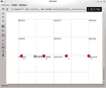
In the simulation script netanim1.cc the line std::string animFile = netanim1.xml; creates an animation trace file with the name netanim1.xml. After generating the topology, the line d.BoundingBox(1, 1, 25, 25); defines the Cartesian coordinates of the animation window. The line AnimationInterface anim(animFile); sends the data to the file netanim.xml required by NetAnim for displaying the topology animation. Finally, the line anim.EnablePacketMetadata(); adds packet metadata related information to the animation trace file. This line of code is optional. When you execute the ns-3 script, the file netanim1.xml is generated in the directory ns/ns-allinone-3.22/ns-3.22. Now open this file in the NetAnim window by clicking the file menu, and after opening the file, start the topology animation by pressing the Play button. Figure 1 shows the network traffic in the NetAnim window.
If you observe the NetAnim window carefully, you will see different icons denoting operations like start, stop, reload, display packet metadata, zoom in, zoom out, etc. Play around with those buttons for some time till you feel confident about working with NetAnim. The top right corner displays the current simulation time. The speed of the animation can be increased or decreased by moving a button to the left or right. This button is placed at the top panel between the words fast and slow. If you observe Figure 1, you will see that I have reduced the speed of the animation to the minimum possible value to take the screenshot. Now that we have some knowledge of NetAnim, it is time to deal with the ASCII trace files.
ASCII trace files demystified
The three important aspects of ns-3 are simulating the correct topology, understanding the structure of an ASCII trace file, and making changes to the existing ns-3 source files to suit your proposed protocol or architecture. In ns-3, almost all the information is available in the form of an ASCII trace file. Getting results from an ns-3 simulation involves deciphering the trace file. The simulation script netanim1.cc also produces an ASCII trace file named netanim1.tr. The lines of code AsciiTraceHelper ascii; and pointToPointEndNode.EnableAsciiAll(ascii.CreateFileStream(netanim1.tr)); are responsible for generating the trace file. The trace file netanim1.tr is a large file with a number of lines of data. Each line in the trace file corresponds to a trace event. Trace events denote what happens to a packet in the transmit queue of a node. The important events happening in the transmit queue include packet enqueuing denoted by +, packet dequeuing denoted by -, packet reception denoted by r and packet drop denoted by d. Those who are familiar with ns-2 might remember that these symbols carry the same meaning in ns-2 also. Now consider the code shown below. It is actually a single line of data from the trace file netanim1.tr divided into a number of lines for better understanding.
+
2.03474
/NodeList/1/DeviceList/0/$ns3::PointToPointNetDevice/TxQueue/Enqueue
ns3::PppHeader (
Point-to-Point Protocol: IP (0x0021))
ns3::Ipv4Header (
tos 0x0 DSCP Default ECN Not-ECT ttl 63 id 0 protocol 17 offset (bytes) 0 flags [none]
length: 1052 192.169.100.1 > 192.168.100.1)
ns3::UdpHeader (
length: 1032 49153 > 5000)
Payload (size=1024)
As mentioned earlier, the trace event shown above corresponds to a packet enqueue operation because the line starts with the symbol +. The second line tells us the time at which the event happened. The third and fourth lines tells us about the node and device in which the event happened. We now know that the event happened in Device 0 of Node 1. Lines 5 and 6 tell us that a point-to-point protocol is used in this example. Lines 7 to 10 tell us about the IPv4 header details used in this example. We also get the IP addresses of the node from which the packet originates and the node to which it is destined. In this case, the packet originates from a node with IP address 192.169.100.1 and is destined to a node with IP address 192.168.100.1. Lines 11 and 12 tell us that about the UDP header. The thirteenth line tells us about the size of the payload. In this example, the size of the payload is 1024 bytes.
So now we have some idea about the data provided by the trace file netanim1.tr. But alas, the structure of a trace file is not always uniform. When a simulation involves different protocols and different applications, the resulting trace file also varies. So it is not possible to have a single formula to understand the different fields of an ns-3 trace file. Understanding the meaning of the different fields of an ns-3 trace file is one of the skills you have to acquire in the long journey to master ns-3. But whatever the structure of the trace file is, it will contain a number of fields representing some physical parameter. All you have to do is find out which field represents which physical parameter. But even then, you need some tools to analyse the trace file. The next section briefly discusses a few techniques to extract information from a trace file.
Tools to process trace files
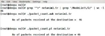
Sometimes, there are millions of lines of data in the trace file. Then, manual processing becomes impossible. In such situations, we have different techniques to extract information from the trace file. Let us consider the simple problem of finding the number of UDP packets received at node 2, the receiver node. We will solve this problem using different approaches. One possible method is to use Linux commands. Highly useful Linux commands for text processing include grep, cut, paste, etc. The grep command is used to select lines from a text containing a particular pattern. The cut command is used to extract specific columns of data from a multi-column data file. The command paste is used for creating multi-column output files, especially useful for producing graphs. Now consider the one-liner given below.
grep ^r netanim1.tr | grep NodeList/2 | wc -l
This will give you the number of packets received at node 2. Here, we use pipelined Linux commands. First, we select all the lines starting with the letter r the event corresponding to packet reception from the trace file. Then from this, we select the lines containing the pattern /Node/2. And finally, we count the number of selected lines with the command wc l. But it may not always be possible to extract information using Linux commands alone. In many situations we need more powerful tools. One such tool is a programming language called AWK, optimised for text processing. Consider the AWK script packet_count.awk given below.
#!/bin/awk -f
BEGIN {
count = 0;
}
{
if($1 == r && $3 ~ /NodeList\/2\//)
{
count++;
}
}
END {
print \n\tNo of packets received at the destination = ,count,\n\n;
}
This AWK script, when executed, will give you the number of packets received at node 2. In an AWK script, the BEGIN section will be processed only oncein the beginning. The END section will also be executed just once at the end. The code given between BEGIN and END sections, enclosed inside the curly bracket, will be executed on every line of the trace file being processed. Each line is divided into a number of fields with whitespace as the character deciding the ending of a field and the beginning of a new field. In the script, $1 contains the first column and this column denotes the event type. $3 contains the third column of the trace file and this corresponds to the third line of the trace file sample shown earlier. So the AWK script selects only those lines that denote a packet reception event at node 2. A counter is incremented if such an event happens and, finally, this value is displayed in the END section.
Even though the language AWK is highly suitable for text processing, its popularity has been waning over the years. As far as text processing is concerned, a general-purpose language called Perl has now taken centre stage. It will be highly beneficial in the long run if you select Perl rather than AWK for text processing. Given below is a Perl script packet_count.pl for finding the number of packets received at node 2.
#!/bin/perl
$infile=$ARGV[0];
open (DATA,<$infile) || die File $infile Not Found;
$counter=0;
while(<DATA>) {
@x = split( );
if($x[0] eq r)
{
if($x[2] =~ /NodeList\/2/)
{
$counter=$counter+1;
}
}
}
printf \n\tNo of packets received at the destination = %d \n\n, $counter;
close DATA;
exit(0);
The working of the Perl script is similar to that of the AWK script. In the script given above, @x is an array variable containing a line of data from the trace file. The variable $x[0] contains the first field of a line of data, which is regarding the event type. Similarly, $x[2] contains the third column of the trace file, and this corresponds to the third line of the trace file sample. Thus the Perl script also counts and reports the number of packets received at node 2. The execution of the three different scripts discussed in this section is shown in Figure 2.
But the scripts will get executed only if your system contains executable files of Perl and AWK. Open a terminal and execute the command echo $PATH. A number of directory names with a complete paths will be displayed. Make sure that the executable files of AWK and Perl are available in any one of these directories. The executable files are named awk and perl. If your system doesnt have these files, install AWK and Perl.


