The distribution of electric supply generally faces a few problems. The good news is that these problems can be modelled mathematically and studied without any danger to life and limb. Gridlabd is open source software which enables smart grid studies.
Economising the operation of electricity generators is a problem (called the ‘economic dispatch problem’) that has been faced since the 18th century. Mathematical models have been developed to study such problems. Another problem is the transmission of power from the generator to the customer, which is called ‘optimal power flow’. The third is the ‘unit commitment problem’, which refers to finding the least-cost ON/OFF state of the available power generation resources to meet the electrical load.
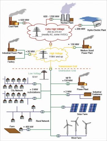
Economising power system operations is still a problem; hence, the term ‘smart grid’. A smart-grid is capable of modelling and studying each device connected to the distribution system, which is highly inefficient compared to generation and transmission systems. Therein lies the importance of Gridlabd software. Gridlabd is capable of modelling each and every component in the power system with mathematics running in its core. It is possible to simulate time-series characteristics from micro-seconds to years. Hence, various cases can be studied on a computer before actual system implementation. It helps in improving the efficiency of an existing system and the future expansion of the distribution system. Figure 1 (courtesy Wikipedia) shows a typical power system network.
Gridlabd (GLD)
Gridlabd was developed by the US Department of Energy (DOE) at Pacific Northwest National Laboratory (PNNL) under funding from the Office of Electricity. While writing this article, the source code for Gridlabd was not available in Ubuntu (am presuming you’re a Debian user). So the available Red Hat package manager (rpm) has been converted to Debian (Deb). Gridlabd is the first simulation platform in which modern energy systems are inbuilt. Time series simulation and load modelling become easier with Gridlabd from sub-station to customers (residential load). Gridlabd is an open source tool freely available to anyone. It encourages collaboration with industry and academia. The BSD-style licence allows us to add or extract our own modules without compromising the internal intellectual property. The Web portal http://www.gridlabd.org/gldportal has a GUI for quick real-time hands-on operation of Gridlabd.
Installation and how it works
Since Gridlabd is not readily available for installation in Ubuntu, we need to convert the available rpm package to Deb. The steps to be followed are given here.
Open a terminal and download the package
hithu@linux:$ wget https://sourceforge.net/projects/gridlab-d/files/gridlab-d/Last%20stable%20release/gridlabd-3.2.0-1.x86_64.rpm.
After downloading, you can check the downloaded file in your home directory. To convert it to a Deb file, you need to install the alien package, as follows:
hithu@linux:$ sudo apt-get install alien
Convert the rpm to Deb by using the command given below:
hithu@linux:$ alien gridlabd−3.2.0−1.x8664.rpm
Exit the terminal. Right-click and open the newly generated Debian file using the Ubuntu software center package manager to complete the installation.
Check the installation by using the following command:
hithu@linux:$ gridlabd --version
GridLAB-D 3.2.0-5368 (Jojoba) 64-bit LINUX RELEASE
To try a simulation of residential temperature variations for a year, save the code given below as residential.glm using a text editor (gedit):
clock {
starttime '2017-02-01 00:00:00 UTC';
stoptime '2018-02-01 00:00:00 UTC';
}
module residential;
module tape;
object house {
object recorder {
property air_temperature;
file temperature.csv;
};
}
In terminal, run the file:
asgridlabd residential.glm
To see output:
more temperature.csv
2017-02-01 00:00:00 UTC,+72.4767
2017-02-01 01:00:00 UTC,+73.5292
2017-02-01 02:00:00 UTC,+74.1789
2017-02-01 03:00:00 UTC,+74.7188
2017-02-01 04:00:00 UTC,+75.1863
2017-02-01 05:00:00 UTC,+75.6680
2017-02-01 05:24:12 UTC,+76.0000
2017-02-01 05:29:10 UTC,+73.9968
2017-02-01 06:00:00 UTC,+75.9057
2017-02-01 06:02:18 UTC,+76.0006
2017-02-01 06:07:40 UTC,+73.9994
2017-02-01 06:25:12 UTC,+76.0006
2017-02-01 06:30:33 UTC,+73.9961
2017-02-01 06:48:21 UTC,+76.0001...
Hence, you have the result of temperature variations in a typical house with hourly intervals, for a year. It is possible to change the interval, add the location of meteorological data, measure various parameters, add more implicit devices, and much more.
There are many modules available within this software:
gridlabd --modhelp residential
The module given above the list of the various classes and objects possible in a residential simulation. For example, class ‘freezer’ has…
class freezer {
parent residential_enduse;
class residential_enduse {
loadshape shape;
enduse load; // the enduse load description
complex energy[kVAh];
// the total energy consumed since the last meter reading
complex power[kVA];
// the total power consumption of the load
complex peak_demand[kVA];
// the peak power consumption since the last meter reading
double heatgain[Btu/h];
// the heat transferred from the enduse to the parent
double cumulative_heatgain[Btu];
// the cumulative heatgain from the enduse to the parent
double heatgain_fraction[pu];
// the fraction of the heat that goes to the parent
double current_fraction[pu];
// the fraction of total power that is constant current
double impedance_fraction[pu];
// the fraction of total power that is constant impedance
double power_fraction[pu];
// the fraction of the total power that is constant power
double power_factor; // the power factor of the load
complex constant_power[kVA];
// the constant power portion of the total load
complex constant_current[kVA];
// the constant current portion of the total load
complex constant_admittance[kVA];
// the constant admittance portion of the total load
double voltage_factor[pu];
// the voltage change factor
double breaker_amps[A]; // the rated breaker amperage
set {IS220=1} configuration; // the load configuration options
enumeration {OFF=4294967295, NORMAL=0, ON=1} override;
enumeration {ON=1, OFF=0, UNKNOWN=4294967295} power_state;

}

double size[cf];
double rated_capacity[Btu/h];
double temperature[degF];
double setpoint[degF];
double deadband[degF];
timestamp next_time;
double output;
double event_temp;
double UA[Btu/degF*h];
enumeration {ON=1, OFF=0} state;
}
Further detailed documentation on power flow analysis is given on the website http://gridlab-d.sourceforge.net/wiki/index.php/Powerflow. More technical help on the software can be accessed at https://sourceforge.net/p/gridlab-d.
Accurate modelling of distribution networks and connected devices is possible with this open source software. The only drawback is that the original software doesn’t have a GUI. It can be used as a benchmark for comparison between various systems. Results obtained can be plotted and interpreted using other open source software like Scilab, LibreOffice Calc, etc. Kindly refer to my article in the February 2017 issue of OSFY. As of now, Gridlabd has the flexibility for smart-grid simulation.


