


David H. Hubel and Torsten Wiesel laid the foundations for building the CNN (convolutional neural network) model after their studies and experiments on the human visual cortex. Since then, CNN models have been built with near human accuracy. This article explores image processing with reference to the handling of image features in CNN. It covers the building blocks of the convolution layer, the kernel, feature maps and how the activations are calculated in the convolution layer. It also provides insights into various types of activation feature maps and how these can be used to debug the CNN model to reduce computations and the size of the model.
“More than 50 per cent of the cortex, the surface of the brain, is devoted to processing visual information,” said William G. Allyn, a professor of medical optics.
The human visual cortex is approximately made up of around 140 million neurons. In addition to other tasks, this is the key organ responsible for detecting, segmenting and integrating the visual data received by the retina. It is then sent to other regions in the brain where it is processed and analysed to perform object recognition and detection, and subsequently retain it as applicable.
In the early 1950s, David H. Hubel and Torsten Wiesel conducted a series of experiments on cats and won two Nobel prizes for their amazing findings on the structure of the visual cortex. They revolutionised our understanding of the human visual cortex and paved the way for much further research based on this topic.
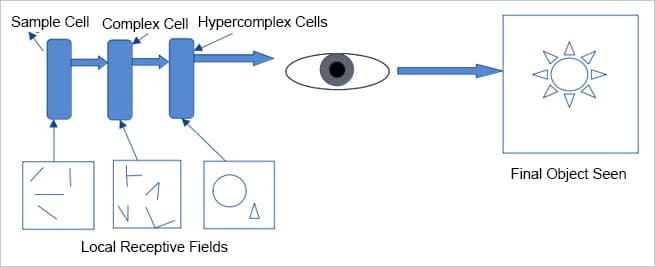
Their studies showed that in the visual cortex, many neurons have small local receptive fields. A local receptive field means that these neurons react to visual stimuli only if they are located in a specific region of the visual field of perception. In other words, these neurons are fired or activated only if the visual stimulus is located at a particular place on the retina or visual field. They found that some neurons have larger receptive fields and they are fired, activated or react to complex features in the visual field, which in a way are a combination of low-level features to which other neurons react. The low-level features mean horizontal and vertical lines, edges and corners and different angles of lines, while high-level features are the simple or complex combinations of these low-level features. Figure 1 illustrates the local receptive fields of different cells in the human visual cortex.
Hubel and Wiesel also discovered that there are three types of cells in the visual cortex and each has distinct characteristics, based on the features they learn or react to. These are: simple, complex and hyper-complex. Simple cells are responsible for learning basic features like lines and colours; complex cells for learning features like edges, corners and contours, while hyper-complex cells are responsible for learning combinations of features learnt by simple and complex cells. This powerful insight paved the way to understanding how perception is built – the receptive fields of multiple neurons may overlap and together they tile the whole field. These neurons work together, with a few neurons learning features on their own and others learning by combining the features learnt by other neurons, and finally integrating to detect all forms of complex features in any region of the visual field.
For the video of the Hubel and Wiesel experiment, visit https://www.youtube.com/watch?v=y_l4kQ5wjiw.
CNN architecture
CNNs are the most preferred deep learning models for image classification or image related problems. Of late, CNNs have also been used to handle problems in fields as diverse as natural language processing, voice recognition, action recognition and document analysis. The most important characteristic of CNNs is that they automatically learn the important features without any guided supervision. Given the images of two classes, for example, dogs and cats, a CNN will be able to learn the distinctive features of dogs and cats by itself.
Compared to other deep learning models for image related problems, CNNs are computationally efficient, which makes them the preferred option since they can be configured to run on many devices. Ever since the arrival of AlexNet in 2012, researchers have successfully built new CNN architectures that have very good accuracy, with powerful and efficient models. Popular CNN model architectures include VGG-16, Inception models, ResNet-50, Xception and MobileNet.
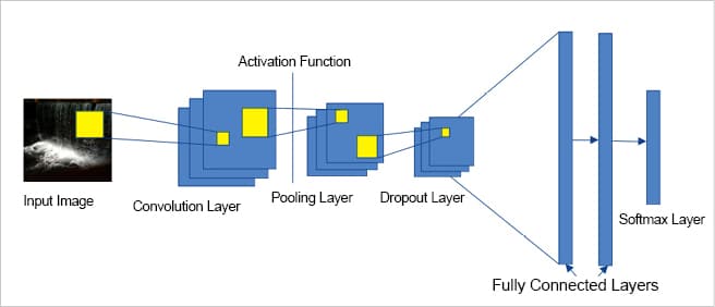
In general, all CNN models have architectures that are built using the following building blocks. Figure 2 depicts the basic architecture of a CNN model.
- Input layer
- Convolution layers
- Activation functions
- Pooling layers
- Dropout layers
- Fully connected layers
- Softmax layer
In the CNN architecture, the building blocks involving the convolution layer, activation function, pooling layer and dropout layer are repeated before ending with one or more fully connected layer and the softmax layer.
Convolution layer
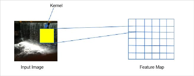
The convolution layer is the most important building block of the CNN architecture. The neurons in the first convolution layer are not connected to all the pixels in the input image, but are connected to pixels of their local receptive fields, as shown in Figure 2. Mathematically, the convolution layer merges two sets of information to produce a feature map. It applies the convolution filter or
kernel to the input and produces the feature map. Let us understand this better with an example.
Let us suppose that the input image size is 6 x 6 and the kernel size is 3 x 3. To draw a parallel to the visual cortex, the visual field size is 6 x 6 and the local receptive field size is 3 x 3. To generate the feature map, the kernel is made to slide over each pixel location of the input image. Hence a single value is generated for each convolution operation (the summation or multiplication of the pixel value with the corresponding kernel value in the same location). The area on the input image that is used during each convolution operation is the receptive field, the size of which is equivalent to the kernel size. Since the kernel is made to slide over the entire input image, an equal-sized feature map as the input image is produced after the convolution operation is applied to the entire image. The same procedure is followed for 3D images or multi-colour channel input images. An independent feature map is also produced for each channel in that case. Since there is one feature map for each convolution operation using a kernel, for a normal 2D image in grey scale, the number of feature maps produced in each layer is equal to the number of kernels used at that layer. For 3D images, it is three times the number of kernels due to three colour channels.
During a convolution operation, for each row x and column y in the feature map, the value at position (x, y) will be the total of the multiplication of values in rows x to:
x + kh – 1, columns y to y + kw – 1
…where kh and kw are the height and width of the receptive fields. Hence, to produce a feature map equal to the input image size, suitable padding has to be done around the input image. In general, zero padding is applied to the input image.
It is also possible to slide the kernel over the input image by spacing out the pixel location. That means, as described above, the kernel is made to slide over each pixel location of the input image to generate the feature map. The distance between each successive receptive field is one (based on pixel locations). The spacing out or distance between two successive receptive fields is called the stride. As the kernel is made to slide over rows and columns, the stride can be different for sliding across rows (vertical direction) and columns (horizontal direction). With the stride value more than one, it is possible to produce a feature map that is smaller than the input size. With the stride, the neuron value in the feature map located at (x, y) is produced by rows.
(x) * sh + kh - 1, columns (y) * sw + kw – 1,
…where sh and sw are horizontal and vertical strides.Each location (x, y) in the feature map will be a neuron generated using the specific kernel in that convolution layer. The neuron’s weight at a location (x, y) will hence be a value, after the convolution operation is applied to rows x to:
x + kh – 1, columns y to y + kw – 1,
…where kh and kw are the height and width of the receptive field of the input. The CNN model is built to learn the equation WX + b, where W is the weight of the neurons, X is the activation values of neurons, and b is the bias term. All neurons in a feature map share the same weights (kernel) and bias term, but different activation values that correspond to the values of the receptive field corresponding to that neuron in the feature map. This is one of the reasons why computations are less in a CNN compared to a DNN (deep neural network). A feature learnt by a neuron at one particular location will allow it to detect the same feature anywhere else in the input, regardless of the location. This is another important feature of the CNN as compared to a DNN, which is not translational invariant.
Next, consider the convolution layers after the first convolution layer. The neuron at location (x, y) in the feature map k in a convolutional layer l gets its input from all the neurons in the previous layer l -1, which are located in rows:
x * sw to * sh + kw - 1, columns y * sh to y * sw + kh – 1
…and for all feature maps in the layer l – 1. These are the same inputs to all neurons located in the same row x and column y, in all the feature maps. This explains how the features learnt in one layer get integrated to learn combined features or complex patterns in successive layers. This also explains how a CNN learns distinct features at the initial layers; and convolutes to integrate basic features to learn complex distinct features or patterns in the intermediate convolution layers, before finally learning objects present in the input in the last convolution layers. As discussed earlier, any feature, pattern or object learnt by the CNN at any layer will allow it to detect this anywhere else in the input, independent of the location. So one needs to be extra careful when using a CNN to detect combined objects that are similar in the input. For example, in the case of face detection, if one is interested in studying the features of the eye and eyebrows together as a combination, then normal CNN would learn the features of the eyebrow and the eye as two different features, and it may not help in learning the minor differences of the combination of features. In that case, the convolution layers have to be tweaked to learn those features appropriately.
Activation feature maps in CNN
Although activations are generated for each neuron, they may not be propagated to the final prediction. Let us now get the equations to determine the output of a neuron at a convolutional layer. For a grey scale image (single channel) the output of the neuron in the first convolution layer located at (x, y) of the feature map k is given by the following:
zx, y = Σm=1 to kh (Σn=1 to kw (ai, j * wm,n)) + bk for i = m * sh + kh – 1 and j = n * sw – 1 and ai, j
…which will be the pixel values of the input image. And by:
kh, kw, sh, and sw
…which are the height and width of the kernel and the horizontal and vertical strides, respectively.The output of the neuron in any convolutional layer l (l is not the first convolutional layer) and for the feature map k is given by the following:
zx, y, k = Σm=1 to kh (Σn=1 to kw (Σfm = 1 to kl-1 (ai, j, fm * wm, n, fm, k))) + bk for i = m * sh + kh – 1 and j = n * sw – 1 and ai, j, fm
…which will be the activation values of previous layer l – 1. And by:
kh, kw, sh, and sw
…which are the height and width of the kernel, and the horizontal and vertical strides, respectively.
zx, y, k
The above is the output of the neuron located at row m, column n in the feature map k of the convolutional layer l.
kl-1
The above is the number of feature maps in the layer l-1 (previous layer).
ai, j, fm
The above is the activation output of the neuron located in layer l – 1, row i, column j, and feature map fm. bk is the bias term for feature map k (in layer l).
wi, j, fm, k
The above is the weight (kernel) of any neuron in the feature map k of the layer l and its input located at row m, column n, relative to the neuron’s receptive field and feature map fm.
The feature maps produced in the convolution layer are input to the next layer (pooling layer) after applying the activation function. The feature map generated after applying the activation function is called the activation feature map. The visualisation of the activation feature map for a filter in a particular convolution layer depicts the regions of the input that are activated in the feature map after applying the filter. In each activation feature map, the neurons have a range of activation values with the maximum value representing the most activated neuron, the minimum value representing the least activated neuron, and the value zero representing a neuron not activated.
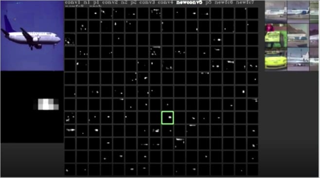
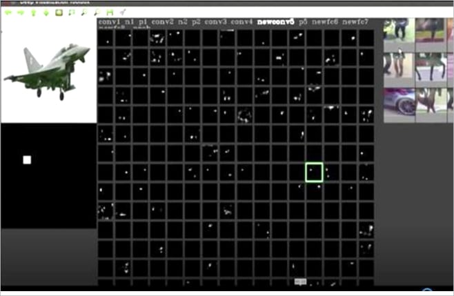
Let us consider an illustration. The AlexNet model is used for transfer learning to build a binary classifier that classifies the given flight image to either a passenger flight or a fighter flight. AlexNet has five convolutional layers — the first four convolutional layers are frozen and the model is trained to obtain very good accuracy of around 98 per cent. The figures 4 and 5 show the visualizations of the activation feature maps of the fifth convolutional layer, which has 256 filters and hence 256 activation feature maps. Figures 4 and 5 show the following details.
- The activation feature maps for the passenger flight image and the fighter flight image for the newconv5 convolution layer (the fifth convolutional layer of the AlexNet model, renamed to newconv5 since it has been retrained during transfer learning).
- The passenger and fighter flight test images (top left corner in the figure) for which visualisations are shown.
- Assume the activation feature maps are arranged as a 16 x 16 matrix with index 1 given for activation feature map at row 1, column 1; and index 17 for the activation feature map at row 2, column 1, and so on.The higher resolution image of the selected activation feature map (green coloured box) is shown just below the test image.
In Figure 4, check the 137th activation feature map (the green coloured box), which is shown as a high resolution image below the test image. The white coloured pixels in this image show only those features that have been learnt by this filter or, in other words, these are the activated neurons of the feature map with a value greater than zero. The remaining pixel values are zero and hence black in colour, so neurons corresponding to those pixels are not activated. From a comparison between the activation feature map and the original image, it can be seen that the features in the activation feature map correspond to multiple windows in the input image. This can also be justified by checking the top nine highly activated images shown at the top right corner in the figure. The top nine images show the objects that have multiple window patterns or features. Refer to http://yosinski.com/deepvis for more details on visualisation of the CNN model. A similar analogy is applicable to neurons in all the feature maps shown above.
Now, among the 16 x 16 activation feature maps in the convolution layer shown in Figures 4 and 5, it can be seen that many of these maps are not showing any activations. None of the neurons in these feature maps are activated. CNN theory states that each filter represents distinct feature/s at each layer, and in these figures, each of the 256 filters represents features of the passenger or the fighter flight that are learnt. If there are no activations, this means that it does not learn any feature. Since the model is a binary classifier for classifying passenger and fighter flights, each of the filters in the convolution layer will be learning either passenger or fighter features. Hence these feature maps can be classified into four types – class 0, class 1, mixed and inactive.
- Class 0: In these feature maps, the features learnt belong to class 0 only.
- Class 1: In these feature maps, the features learnt belong to class 1 only.
- Mixed: In these feature maps, the features learnt belong to both class 0 and class 1.
- Inactive: These feature maps do not learn any features of class 0 or class 1.
The type of activation feature maps in each layer can be easily visualized using the Deepvis tool specified above. Many a times, complex standard models are used to build a simple binary as above, or a model for up to ten class classifiers using transfer learning. During those scenarios, as seen above, many filters may not be required since they will not be learning any features at all, and fewer filters will be sufficient to learn features of all the classes. In these cases, if the requirement is to retain the original model architecture for some reason, then the inactive filters can be removed to reduce the computations and the size of the model.
The types of filters will also help to debug when the test image is mis-classified. The types of filters at each layer can be studied for both the classes during training and during evaluation. The filters activated can be compared during training and evaluation. When making a correct prediction of the test image, the count of the type of filters for each class will approximately match the average count of the type of filters for each class during training. This means that if a test image is correctly classified as a passenger flight class, then its count of the type of filters (class 0, class 1, mixed and inactive) must be approximately equal to the average count of the type of filters of the passenger flight determined during training, and the same will be true for an image correctly classified as the fighter flight class.
These findings can help to debug mis-classified images. For example, if the test image is mis-classified as the fighter class, then the count of the type of filters will not match the count of the type of filters for the fighter class during training, which is quite obvious. The potential reason for mis-classification could be any of the following:
The model has evaluated the features of both the fighter and passenger flight classes, and found that fighter features dominating the passenger features during classification and hence it is mis-classified.
The model has evaluated and found more of fighter features matching during classification and hence it is mis-classified.
The model has evaluated and found comparable fighter and passenger features matching during classification and due to minor differences in features learnt, it has been mis-classified
To understand the above reasoning, the activation feature maps of each convolution layer need to be analysed, and the average count of the type of filters at each layer may have to be considered to come to a conclusion. There are approaches to handle this, which will be discussed in the next article.
This article provides an overview of how the visual cortex perceives objects. It explains the parallels between CNNs and different building blocks of the CNN architecture. It also briefly covers each building block and how the convolution layer processes the image features from the input. It then highlights the importance of activation during image classification. Knowing the details about the activations of each filter in each layer allows model developers to understand the importance of each filter and update their CNN architectures or build new CNNs with reduced parameters and computations. The article also gives details on the types of activation feature maps, and how they can be used for debugging CNN models and to detect potential mis-classification. Further exploration and research on activation feature maps for different types of models other than CNN will provide many insights, especially for object detection and recognition models. The same can be extended to natural language processing and voice recognition models, the activation feature maps for which would be a bit more complex to analyse.


