

This two-part series of articles explains and demonstrates how to implement a recommender system for an online retail store using Python. The first part of the series, published in the May 2022 issue of Open Source For You, focused on the theory behind such a system. This second part explains how to implement that system.
The data set used for research can be found and accessed via https://data.world/uci/online–retail. Its details are given in the box below.
Solution methodology
So how does one create a system that recommends a specific number of products to users on an e-commerce website, based on their previous purchase history. To construct the answer, we employed the Skip-Gram modelling technique of the word2vec algorithm that we have seen in Part 1. However, we took a customer-focused approach to this.
| Source Dr Daqing Chen, Director: Public Analytics Group (chend ‘@’ lsbu.ac.uk), School of Engineering, London South Bank University, London.Data set information This is a transnational data set that contains all the transactions occurring between 01/12/2010 and 09/12/2011 for a UK based and registered non-store online retail. The company mainly sells unique all-occasion gifts. Many customers of the company are wholesalers. Attributes used in the data setInvoiceNo: Invoice number. Nominal — a 6-digit integral number uniquely assigned to each transaction. If this code starts with letter ‘c’, it indicates a cancellation. |
The suggested system incorporates consumer purchasing behaviour as a feature. Word2vec is used to create a vector representation of the products. It provides low-dimensional (50–500) and dense (not sparse; most values are non-zero) word embedding formats. As a result, if a user is browsing a product online, we can immediately suggest related items based on the product’s vector similarity score.
After gathering the necessary data and performing a train-test split on it, an attempt was made to create word and sentence equivalents comparable to those of a standard word2Vec model, which was then fed to the model for training.
We will try and explain the implementation by dividing it in three parts:
- Data pre-processing
- Exploratory data analysis
- Model building
Data pre-processing
We will first take a quick look at the data set in this segment that we are going to evaluate, to see how we can make it easier and more useful for further research.
Let’s get started by importing the necessary libraries and the data set we’ll be working with. Because the ‘InvoiceDate’ attribute is in an unsatisfactory format, we fix it by using this date variable to format our desired type. We also have some wrong spellings and excessive white spaces in our strings that we would like to prevent, and we would like to keep our strings in upper case for the next steps.
We will install openpyxl using the command given below:
!pip install openpyxl

Collecting openpyxl
  Downloading openpyxl-3.0.9-py2.py3-none-any.whl (242 kB)
|████████████████████████████████| 242 kB 4.2 MB/s
Collecting et-xmlfile
  Downloading et_xmlfile-1.1.0-py3-none-any.whl (4.7 kB)
Installing collected packages: et-xmlfile, openpyxl
Successfully installed et-xmlfile-1.1.0 openpyxl-3.0.9
WARNING: Running pip as the ‘root’ user can result in broken permissions and conflicting behaviour with the system package manager. It is recommended to use a virtual environment instead (https://pip.pypa.io/warnings/venv).
Next, we will import the necessary libraries and the data set:
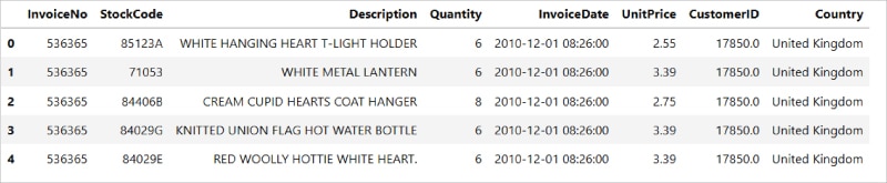
import numpy as np, pandas as pd, re, scipy as sp, scipy.stats

#Importing Dataset
pd.options.mode.chained_assignment = None
datasetURL = ‘https://query.data.world/s/e42xdsj4d3a6evs7t3z6kjkoj4edsl’
df1 = pd.read_excel(datasetURL)
original_df=df1.copy()
original_df.head()
Figure 1 shows the output of the above command.
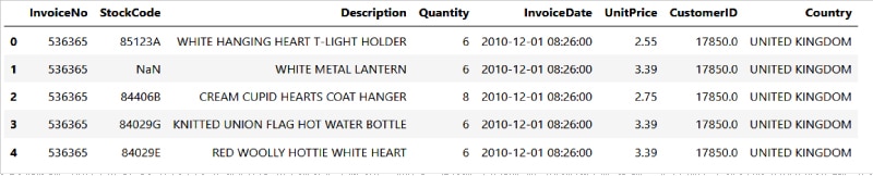
df1.size
df1.isnull().sum().sort_values(ascending=False)
df1=df1.dropna(axis=0)
df1.isnull().sum()
#Formatting Date/Time
df1[‘InvoiceDate’] = pd.to_datetime(df1[‘InvoiceDate’], format = ‘%m/%d/%Y %H:%M’)

Checking the strings

df1[‘Description’] = df1[‘Description’].str.replace(‘.’,’’).str.upper().str.strip()
df1[‘Description’] = df1[‘Description’].replace(‘\s+’,’ ‘,regex = True)
df1[‘InvoiceNo’] = df1[‘InvoiceNo’].astype(str).str.upper()
df1[‘StockCode’] = df1[‘StockCode’].str.upper()
df1[‘Country’] = df1[‘Country’].str.upper()
df1.head()
As intuitive as the variables (column names) may sound, let’s take a step further by understanding what each variable means.
InvoiceNo (invoice_num): A number assigned to each transaction
StockCode (stock_code): Product code
Description (description): Product name
Quantity (quantity): Number of products purchased for each transaction
InvoiceDate (invoice_date): Time stamp for each transaction
UnitPrice (unit_price): Product price per unit
CustomerID (cust_id): Unique identifier for each customer
Country (country): Country name
| Note: Product price per unit is assumed to follow the same currency throughout our analysis. |
By understanding the data in a more descriptive manner, we notice two things:
- Quantity has negative values
- Unit price has zero values (Are these FREE items?)
We have some odd and irregular values in the ‘UnitPrice’ and ‘Quantity’ columns, as seen in the summary of our data set, which we will locate and eliminate to prevent them from negatively affecting our study. We can see that some of the transactions in the ‘StockCode’ variable are not actually products, but rather costs or fees related to the post or bank, or other transactions that we don’t really require in our data. We realise that some of these transactions contain returned products, and that in those transactions, the ‘InvoiceNo’ begins with a ‘c’ character and the ‘UnitPrice’ should be negative. However, we have purchases in our database with negative ‘UnitPrice’ and vice versa, which we need to correct. There are also certain tuples where the ‘UnitPrice’ is left blank. There are many missing or inaccurate values in the ‘Description’ attribute. To resolve this issue, we will delete transactions with no accessible description, check the ‘Description’ based on the product ‘StockCode’, and fill the missing values with the right ‘Description’ that is available from other transactions with the same ‘StockCode’.
Next, we will look for the missing and incorrect values:
df1.drop(df1[(df1.Quantity>0) & (df1.InvoiceNo.str.contains(‘C’) == True)].index, inplace = True)
df1.drop(df1[(df1.Quantity<0) & (df1.InvoiceNo.str.contains(‘C’) == False)].index, inplace = True)
df1.drop(df1[df1.Description.str.contains(‘?’,regex=False) == True].index, inplace = True)
df1.drop(df1[df1.UnitPrice == 0].index, inplace = True)

for index,value in df1.StockCode[df1.Description.isna()==True].items():
    if pd.notna(df1.Description[df1.StockCode == value]).sum() != 0:
        df1.Description[index] = df1.Description[df1.StockCode == value].mode()[0]
    else:
        df1.drop(index = index, inplace = True)

     df1[‘Description’] = df1[‘Description’].astype(str)

#Adding Desired Features
df1[‘FinalPrice’] = df1[‘Quantity’]*df1[‘UnitPrice’]
df1[‘InvoiceMonth’] = df1[‘InvoiceDate’].apply(lambda x: x.strftime(‘%B’))
df1[‘Day of week’] = df1[‘InvoiceDate’].dt.day_name()
df1.shape
The output of the execution will be:
(406789, 11)
Exploratory data analysis
In this section, we will visualise the data to have a clear vision and gain insights into it.
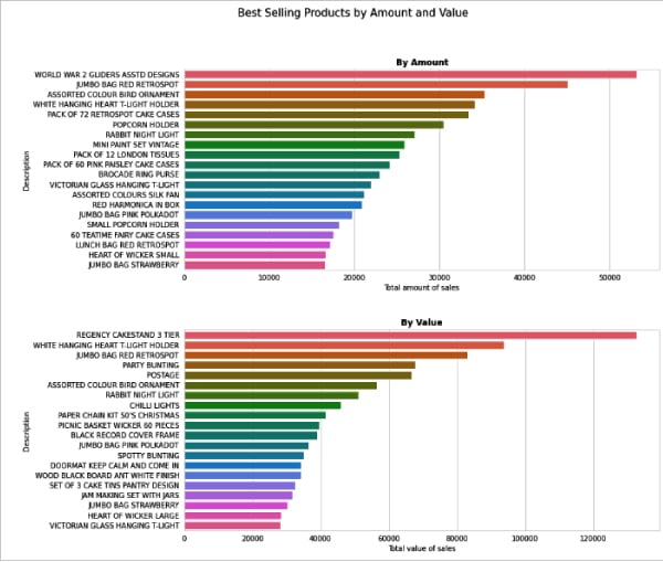
We import our data in this section and update to datetime so that we can work on the data from the time series. We’re going to start by showing what the top items we have sold around the globe are. There are two metrics that can show us how much benefit each product has produced. In the first plot of the subplot below, we can see the top 20 goods purchased by clients with respect to price and in the most quantities.
#importing necessary libraries and the cleaned dataset
import pandas as pd, numpy as np, matplotlib.pyplot as plt, seaborn as sns
%matplotlib inline
Cleaned_Data = df1
Cleaned_Data.index = pd.to_datetime(Cleaned_Data.index, format = ‘%Y-%m-%d %H:%M’)

#top 20 products by quantity and finalprice
sns.set_style(‘whitegrid’)
TopTwenty = Cleaned_Data.groupby(‘Description’)[‘Quantity’].agg(‘sum’).sort_values(ascending=False)[0:20]

Top20Price = Cleaned_Data.groupby(‘Description’)[‘FinalPrice’].agg(‘sum’).sort_values(ascending=False)[0:20]
#creating the subplot
fig,axs = plt.subplots(nrows=2, ncols=1, figsize = (12,12))
plt.subplots_adjust(hspace = 0.3)
fig.suptitle(‘Best Selling Products by Amount and Value’, fontsize=15, x = 0.4, y = 0.98)
sns.barplot(x=TopTwenty.values, y=TopTwenty.index, ax= axs[0]).set(xlabel=’Total amount of sales’)
axs[0].set_title(‘By Amount’, size=12, fontweight = ‘bold’)
sns.barplot(x=Top20Price.values, y=Top20Price.index, ax= axs[1]).set(xlabel=’Total value of sales’)
axs[1].set_title(‘By Value’, size=12, fontweight = ‘bold’)
plt.show()
We can see the output in Figure 3.
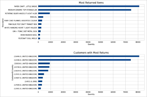
ReturnedItems = Cleaned_Data[Cleaned_Data.Quantity<0].groupby(‘Description’)[‘Quantity’].sum()
ReturnedItems = ReturnedItems.abs().sort_values(ascending=False)[0:10]
ReturnCust = Cleaned_Data[Cleaned_Data.Quantity<0].groupby([‘CustomerID’,’Country’])[‘Quantity’].sum()
ReturnCust = ReturnCust.abs().sort_values(ascending=False)[0:10]

#creating the subplot
fig, [ax1, ax2] = plt.subplots(nrows=2, ncols=1, figsize=(12,10))
ReturnedItems.sort_values().plot(kind=’barh’, ax=ax1).set_title(‘Most Returned Items’, fontsize=15)
ReturnCust.sort_values().plot(kind=’barh’, ax=ax2).set_title(‘Customers with Most Returns’, fontsize=15)
ax1.set(xlabel=’Quantity’)
ax2.set(xlabel=’Quantity’)
plt.subplots_adjust(hspace=0.4)
plt.show()
Now let us find out the items that were returned the most, and the customers with the corresponding country:
Figure 4 shows the graph plotted for the above criteria.
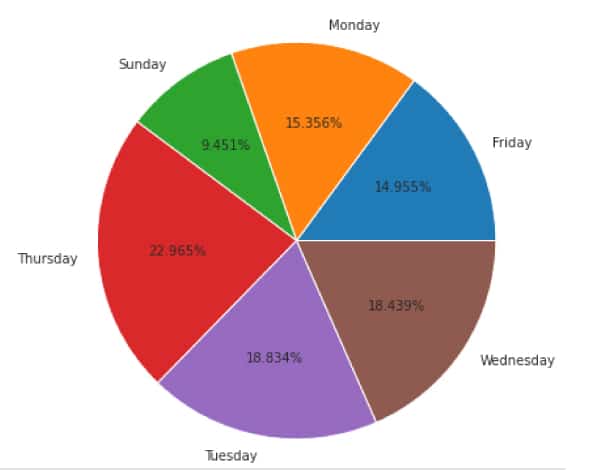
Since we have got the day of the week in which the things were sold, we can use it to see the sales value by each day of the week. We can create the pie chart as shown in Figure 5.
#creating the pie chart
Cleaned_Data.groupby(‘Day of week’)[‘FinalPrice’].sum().plot(kind = ‘pie’, autopct = ‘%.3f%%’, figsize=(7,7)).set(ylabel=’’)
plt.title(‘Percentages of Sales Value by Day of Week’, fontsize = 17)
plt.show()
Model building
Let’s first save the data set to be used in an Excel file, so that we can use it according to our needs.
#Creating an Excel File for the Cleaned Data
Cleaned_Data.to_excel(‘Online_Retail_data.xlsx’)

#Loading the excel file cleaned data into a dataframe
final_data=pd.read_excel(‘Online_Retail_data.xlsx’,index_col=0)
final_data.head()

# convert the StockCode to string datatype
final_data[‘StockCode’]= final_data[‘StockCode’].astype(str)

# List of unique customers
customers = final_data[“CustomerID”].unique().tolist()
len(customers)
The output will be:
4371
Our data set contains 4,371 customers. We will extract the purchasing history of each of these clients. In other words, we can have 4,371 different purchase sequences.
To construct word2vec embeddings, we’ll leverage data from 90 per cent of our clients. The remaining data set will be utilised for validation.
Let’s split the data set.
Train – test data preparation
# shuffle customer ID’s
random.shuffle(customers)

# extract 90% of customer ID’s
customers_train = [customers[i] for i in range(round(0.9*len(customers)))]

# split data into train and validation set
train_df = final_data[final_data[‘CustomerID’].isin(customers_train)]
validation_df = final_data[~final_data[‘CustomerID’].isin(customers_train)]
Now, for both the train and validation sets, we will build sequences of purchases made by customers in the data set.
purchases_train = []

for i in tqdm(customers_train): ## We could have used tqdm(train_df)??
    temp = train_df[train_df[“CustomerID”] == i][“StockCode”].tolist()
    purchases_train.append(temp)
purchases_val = []

for i in tqdm(validation_df[‘CustomerID’].unique()):
    temp = validation_df[validation_df[“CustomerID”] == i][“StockCode”].tolist()
    purchases_val.append(temp)

model = Word2Vec(window = 10, sg = 1, hs = 0,
                 negative = 10, # for negative sampling
                 alpha=0.03, min_alpha=0.0007,
                 seed = 14)

model.build_vocab(purchases_train, progress_per=200)

model.train(purchases_train, total_examples = model.corpus_count,
            epochs=10, report_delay=1)
model.init_sims(replace=True)
model.save(“my_word2vec_2.model”)
Recommending products
To simply match a product’s description to its ID, let’s establish a product-ID and product-description dictionary.
products = train_df[[“StockCode”, “Description”]]

# remove duplicates
products.drop_duplicates(inplace=True, subset=’StockCode’, keep=”last”)

# create product-ID and product-description dictionary
products_dict = products.groupby(‘StockCode’)[‘Description’].apply(list).to_dict()

products_dict[‘90019A’]
The output will be:
[‘SILVER MOP ORBIT BRACELET’]
Let’s create a function which will take a product’s vector (v) as input and return the top six similar products.
def get_similar_item(v, n = 6):

    ms = model.similar_by_vector(v, topn= n+1)[1:]
    my_ms = []
    for j in ms:
        pair = (products_dict[j[0]][0], j[1])
        my_ms.append(pair)

    return my_ms
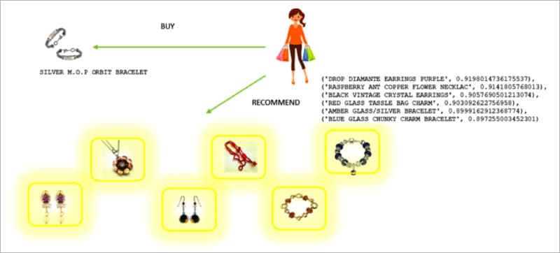
Let’s try out our function by passing the vector of the product ‘90019A’ (‘SILVER M.O.P ORBIT BRACELET’):
get_similar_item(model[‘90019A’])
The output will be:
[(‘TURQUOISE GLASS TASSLE BAG CHARM’, 0.9264411926269531),
 (‘GREEN ENAMEL FLOWER RING’, 0.9179285764694214),
 (‘RED GLASS TASSLE BAG CHARM’, 0.9122185707092285),
 (‘BLUE GLASS CHUNKY CHARM BRACELET’, 0.9082530736923218),
 (‘AMBER DROP EARRINGS W LONG BEADS’, 0.9068467617034912),
 (‘GREEN MURANO TWIST BRACELET’, 0.9062117338180542)]
The above findings are quite relevant and fit the input product well, but the output is only based on a single product’s vector. Let’s work on creating a system that will propose things based on the consumers’ previous purchases. We’ll do this by averaging all the vectors of the products the consumer has purchased so far, and using the resulting vector to discover related things. Create a function that takes a list of product IDs and returns a 100-dimensional vector, which is the mean of the product vectors in the input list.
def my_aggr_vec(products):
    p_vec = []
    for i in products:
        try:
            p_vec.append(model[i])
        except KeyError:
            continue

    return np.mean(p_vec, axis=0)

get_similar_item(my_aggr_vec(purchases_val[0]))
The output will be:
[(‘YELLOW DRAGONFLY HELICOPTER’, 0.6904580593109131),
 (‘JUMBO BAG RED RETROSPOT’, 0.6636316776275635),
 (‘CREAM HANGING HEART T-LIGHT HOLDER’, 0.6594936847686768),
 (‘DISCOUNT’, 0.6384902596473694),
 (‘JUMBO BAG STRAWBERRY’, 0.6319284439086914),
 (“WRAP 50’S CHRISTMAS”, 0.6274842023849487)]

get_similar_item(my_aggr_vec(purchases_val[2]))

[(‘YELLOW DRAGONFLY HELICOPTER’, 0.681573748588562),
 (‘CREAM HANGING HEART T-LIGHT HOLDER’, 0.6654664278030396),
 (‘JUMBO BAG RED RETROSPOT’, 0.6553223133087158),
 (‘WOODEN FRAME ANTIQUE WHITE’, 0.6327764391899109),
 (‘DISCOUNT’, 0.6313808560371399),
 (‘JUMBO BAG STRAWBERRY’, 0.6252866983413696)]
In the end, our system recommended six products based on a user’s complete buying history. The model can also be used to make product suggestions based on recent purchases. Let’s try it with only the previous ten purchases as input:
get_similar_item(my_aggr_vec(purchases_val[0][-10:]))
The output will be:
[(‘YELLOW DRAGONFLY HELICOPTER’, 0.6946737170219421),
 (‘JUMBO BAG RED RETROSPOT’, 0.6675459742546082),
 (‘CREAM HANGING HEART T-LIGHT HOLDER’, 0.6548881530761719),
 (‘DISCOUNT’, 0.6417276859283447),
 (“WRAP 50’S CHRISTMAS”, 0.6357795000076294),
 (‘JUMBO BAG STRAWBERRY’, 0.6348972320556641)]
Summing it up
Word2vec is a fast and powerful method for learning a meaningful representation of words from context. In this article it has been used to solve a shopping-related problem. It enables us to precisely model each product using a vector of coordinates that captures the context in which the product was purchased. This allows us to quickly find products that are comparable for each user.
Suggesting the appropriate products/items to users can enhance not just interaction rates but also product purchases, resulting in increased income. Using machine learning to find similar products also raises product visibility.


