

The KNIME Analytics Platform is open source software built for use in data science. Here’s a short tutorial on how to use it to analyse a FitBit fitness tracker data set to predict the number of calories that will be burnt.
KNIME makes the building of data science workflows and reusable components accessible to everyone by being intuitive, open, and evolving continuously. This article outlines how to make a calorie burn prediction with a random forest predictor through the KNIME Analytics Platform, using a fitness tracker data set.
The KNIME nodes that will be needed for this are listed below: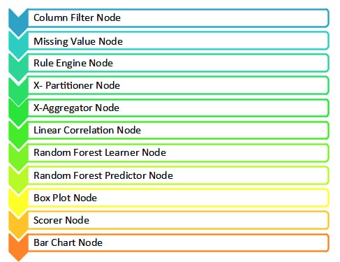
Building the fitness tracker flow
- Download the ‘FitBit fitness tracker data’ data set from https://www.kaggle.com/arashnic/fitbit.
- This data set consists of 15 column attributes, namely: Id, Activity date, Total steps, Total distance, Logged activity distance, Very active distance, Moderately active distance, Light active distance, Sedentary active distance, Very active minutes, Fairly active minutes, Lightly active minutes, Sedentary minutes and Calories. All of the first 14 columns determine the individual’s overall calories burnt in a day. With this data set, we can identify if an individual has a high, low, or good calorie burn for the day.
- Drag and drop the .csv file in the KNIME platform to get the CSV Reader node.
- Connect this with the Column filter and Missing Value node for preprocessing the data. In the Column filter, exclude the ActivityDate column, as the date doesn’t matter for this prediction. In the Missing Value node, enter all the missing values as the mean of the entire column.
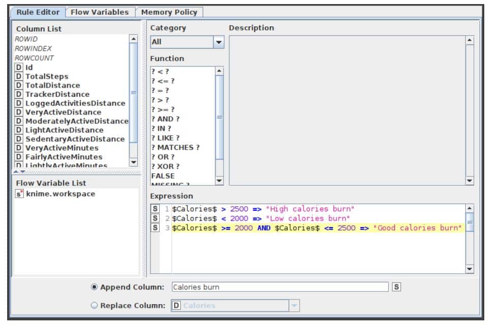
- Connect the Missing Value node with the Rule Engine node. Here, give the rules as follows:
- If Calories > 2500 => High calories burn
- If Calories < 2000 => Low calories burn
- If Calories >= 2000 and Calories <= 2500 => Good calories burn.
- Append this data into a new column named ‘Calories burn’.
6. Connect this with the Box Plot, Linear Correlation and X-Partitioner nodes.
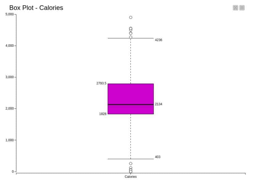
7. In the Box Plot, exclude all the columns except Calories and visualise the plot. We can visualise the robust statistical parameters of minimum, lower quartile, median, upper quartile, and maximum value.
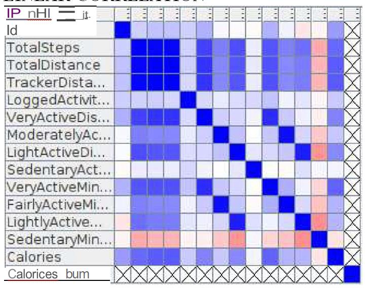
8. The Linear Correlation node calculates a correlation coefficient for each pair of selected columns, i.e., a measure of the correlation of the two variables. Here, all columns are included to calculate the correlation coefficient.
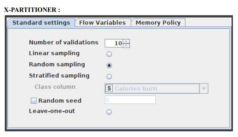
9. The X-Partitioner node is used for performing the cross-validation in the data set. This node is the first in a cross-validation loop. At the end of the loop, there must be an X-Aggregator to collect the results from each iteration. All nodes in between these two nodes are executed as many times as iterations should be performed. We perform 10 validations using random sampling, and the best out of these 10 is given as the output.
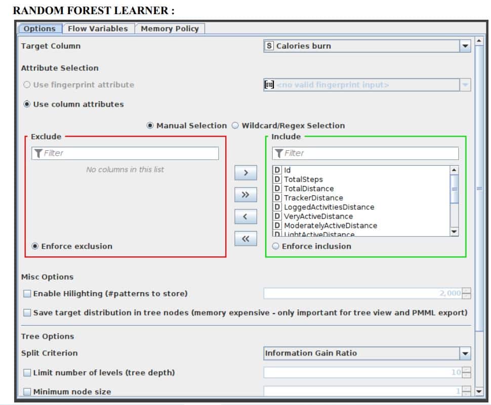
10. Connect the first partition with the Random Forest Learner node. Select the Target column as ‘Calories burn’ and let the rest of the options be the same as the default. Select the split criteria as Information Gain Ratio.
11. Now, connect the Random Forest Predictor node with the second partitioning and the Random Forest Learner node.
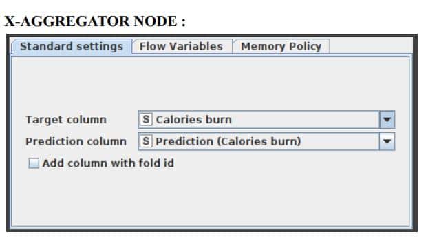
12. Connect this node with the X-Aggregator node. This node collects the result from a Predictor node, compares the predicted class and real class, and outputs the predictions for all rows and the iteration statistics. Select the Target column as ‘Calories burn’ and the Prediction column as ‘Prediction (Calories burn)’.
13. Connect this node with the Scorer and Bar Chart nodes.
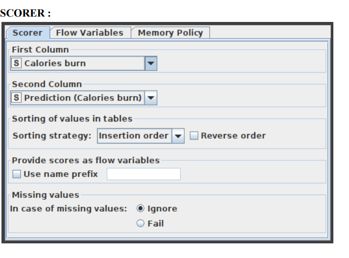
14. In the Scorer node, select the first column as ‘Calories burn’ and the second column as ‘Prediction (Calories burn)’, and save it.
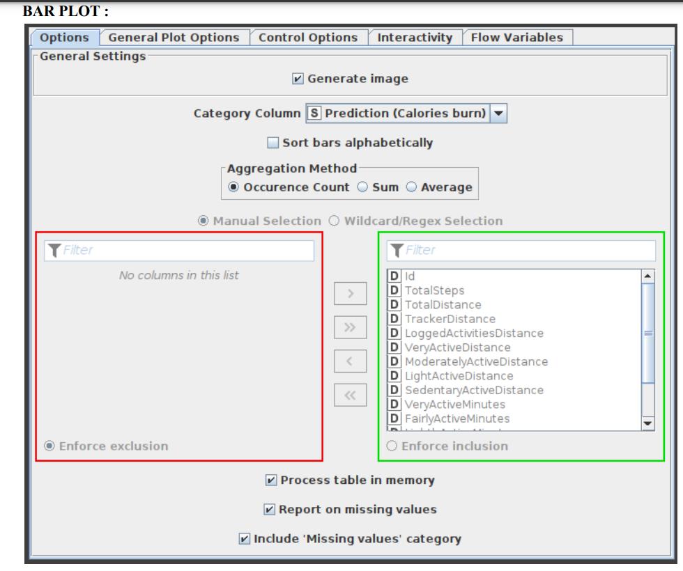
15. In the bar chart, enter the column as ‘Prediction (Calories burn)’, name the chart, and then save it. Finally, execute all the nodes and view the output.
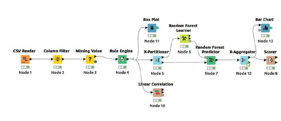
The complete flow for calorie burn prediction using a random forest predictor is given in Figure 1.
Node configurations
Let us see the details needed for node configuration one by one.
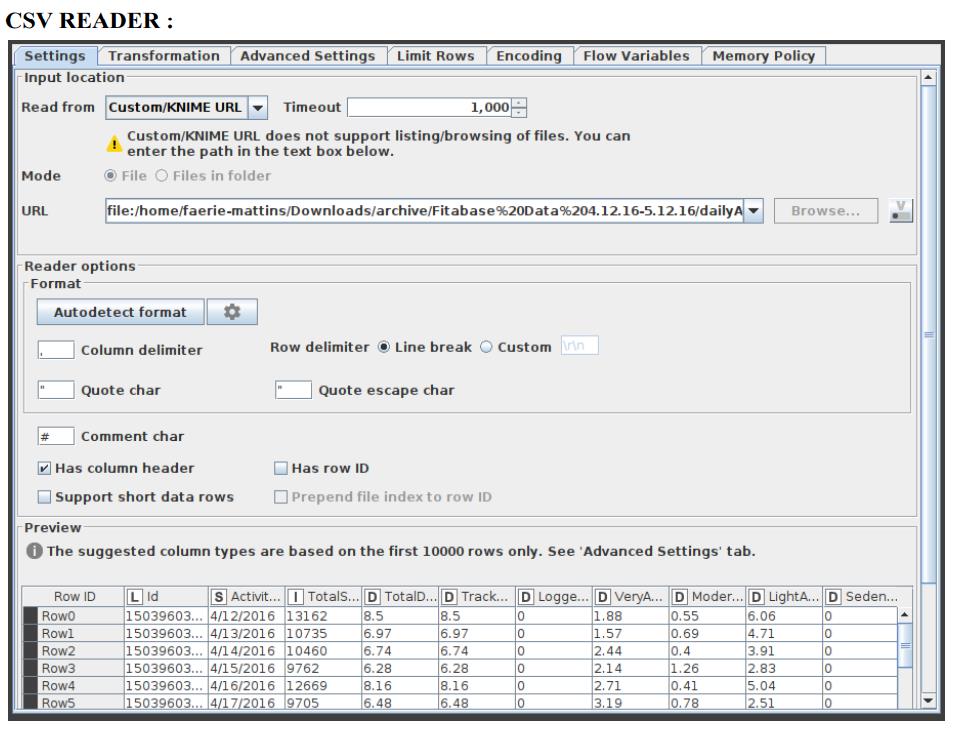
CSV Reader
Figure 2 shows how to configure the CSV Reader.
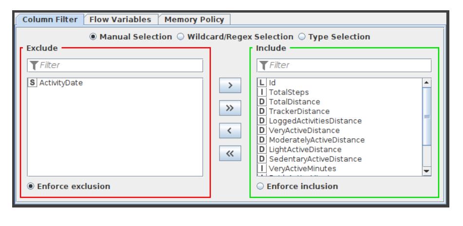
Column Filter
This Column Filter node provides three distinct modes for filtering: manually, by name, and by type. Through Add and Remove buttons, you manually choose which columns to retain and which to exclude. In the name mode, you decide which columns to keep using wild cards and regular expressions. In the type option, you choose which columns to retain based on their type, such as all strings or all integers. The configuration window of this Column Filter node is shown in Figure 3.
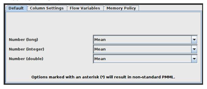
Missing Value
This node aids in handling cells in the input table that have missing values. All columns of a particular kind have default handling options available on the dialog’s first tab, ‘Default’. All columns in the input table that aren’t specifically listed in the second tab, ‘Individual’, have these settings applied to them. Individual settings for each available column are possible using this second tab (thus, overriding the default). Use the second method by selecting the column or group of columns that requires extra treatment, clicking ‘Add’, and then setting the settings. All covered columns in the column list will be selected when you click on the label with the column name(s). Click the ‘Remove’ button for this column to get rid of the extra treatment and replace it with the default handling. Asterisk-denoted options (*) will produce non-standard PMML. A warning will be displayed throughout the execution of the node if you choose this option, and the caution label in the dialogue will turn red. Extensions used by non-standard PMML cannot be read by any software other than KNIME. The configuration window of the missing value node is captured and indicated in Figure 4.
Rule Engine
This node attempts to match a list of user-defined rules to each row in the input table. If a rule is satisfied, the result value is added to a new column. The outcome is determined by the first matching rule in definition order. One line represents each regulation. To insert comments, begin a line with / (comments cannot be placed in the same line as a rule).
Anything following / will not be considered a rule. Rules consist of a condition part (antecedent) that must evaluate to true or false and a consequence (consequent, after the => symbol) that is placed in the new column if the rule matches. A rule’s output may be a string (between “ and /), a number, a Boolean constant, a reference to another column, or the value of a flow variable. The type column represents the common supertype of all potential outcomes (including the rules that can never match). If no rule is applicable, the result is a missing value. Columns are denoted by their respective names surrounded by $, while numbers are presented in the customary decimal format. Note that strings cannot contain (double) quotation marks. $$ TypeCharacterAndFlowVarName $$ is used to represent flow variables. The TypeCharacter for double (real) values should be ‘D’, for integer values ‘I’, and for strings ‘S’. You can manually insert column names and flow variables or use the respective lists in the dialogue. The setup window for the rule engine node is depicted in Figure 5.
X-Partitioner
This node begins the cross-validation loop. An X-Aggregator is required at the conclusion of the loop to collect the results of each iteration. All nodes between these two nodes are run as many times as required by the number of iterations. Figure 6 shows the configuration window for the X-Partitioner node that has been selected for this application.
Random Forest Learner
Minitab, LLC has registered RANDOM FORESTS as a trademark, and its usage is authorised. It consists of a predetermined number of decision trees. Each decision tree model is constructed using a unique collection of rows (records), and for each branch, a random set of columns (describing attributes) is employed. Each decision tree’s row sets are generated using bootstrapping and have the same size as the original input table. The attribute set for a decision tree split is determined by randomly selecting sqrt(m) attributes from the available attributes, where ‘m’ is the total number of learning columns. The properties may also be supplied in bit (fingerprint), byte, or double vector formats. The output model is applied to the associated predictor node and defines a random forest. This node provides a subset of the Tree Ensemble Learner’s capabilities corresponding to a random forest. The configuration window for the Random Forest node that has been chosen for this application can be seen in Figure 7.
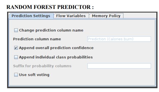
Random Forest Predictor
In a random forest model, this function makes pattern predictions based on an aggregation of the predictions made by the individual trees. Figure 8 displays the settings window for the Random Forest Predictor node.
X-Aggregator
This node must be located at the conclusion of a cross-validation loop and must be the node that comes after an X-Partitioner node. It does this by first collecting the result from a predictor node, then comparing the predicted class to the actual class, and finally outputting the predictions for all rows together with the iteration statistics. Figure 9 illustrates the window for the X-Aggregator node’s configuration options.
Scorer
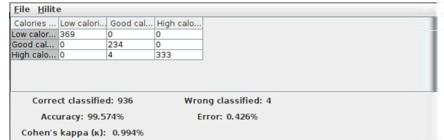
This displays the confusion matrix (the number of rows that share an attribute with their classification) by comparing two columns based on attribute value pairs. You may also highlight cells in this matrix to reveal the underlying rows. The comparison dialogue lets you pick two columns to compare; the rows of the confusion matrix reflect the values in the first column you pick, while the columns reflect the values in the second column. The node returns a confusion matrix where each cell indicates the amount of matches. Statistics on recall, precision, sensitivity, specificity, F-measure, overall accuracy, and Cohen’s kappa are also reported on the second output port. The Scorer node’s settings window is shown in Figure 10.
Bar Plot
Custom CSS styling is supported through a bar char node. The node configuration dialogue allows you to easily condense CSS rules into a single string and set it as the flow variable ‘customCSS’. On KNIME’s documentation page, you can discover a list of the classes that are available as well as their descriptions. Figure 11 exhibits the parameters configuration window for the Bar Plot node.
The results
Now let us see a few of the results.
Scorer node results: The prediction of the calories data set is presented in Figure 12 as the output analysis of the Scorer node.
Linear correlation output: The correlation matrix of the linear correlation analysis is presented in Figure 13.
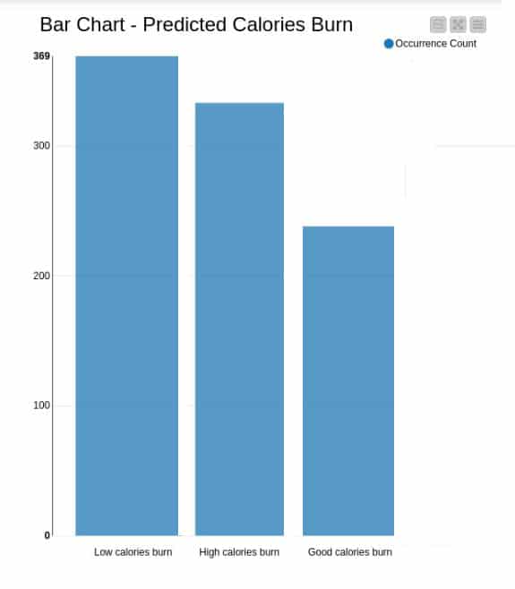
Graphs – bar graph: Appropriate analysis has been made and the bar graph for the predicted calories burn is illustrated in Figure 14. It interprets the occurrence of low calories burn, good calories burn and high calories burn.
Box plot: The box plot for the calories analysis is presented in Figure 15.
Error rate in cross validation: The error rate in cross validations using X-Partitioner and X-Aggregator or 10 validations is depicted in Figure 16.
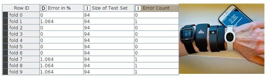
The final accuracy shown by the random forest model is 99.574% and the error is 0.426%. The KNIME Analytics Platform has been successfully used to perform data analysis operations and random forest algorithm on the fitness tracker data set.


