


In this seventeenth article in the R series, we shall learn about linear regression in R.
In statistics, regression is a way to model the relationship between two variables. We will use R version 4.2.1 installed on Parabola GNU/Linux-libre (x86-64) for the code snippets.
$ R --version

R version 4.2.1 (2022-06-23) -- “Funny-Looking Kid”
Copyright (C) 2022 The R Foundation for Statistical Computing
Platform: x86_64-pc-linux-gnu (64-bit)

R is free software and comes with ABSOLUTELY NO WARRANTY.
You are welcome to redistribute it under the terms of the
GNU General Public License versions 2 or 3.
For more information about these matters see
https://www.gnu.org/licenses/.
The mathematical equation for a linear regression between two variables ‘x’ and ‘y’ is defined as ‘y = ax + b’, where ‘a’ and ‘b’ are constants.
The lm() function is used to fit linear models. Consider two vectors ‘x’ and ‘y’ that represent odd and even numbers respectively. We can fit a regression equation between them using the lm() function, as follows:
> x <- c(1, 3, 5, 7, 9)
> y <- c(2, 4, 6, 8, 10)
> r <- lm(y~x)
> print(r)

Call:
lm(formula = y ~ x)


Coefficients:
(Intercept)            x
          1            1
The lm() function accepts the following arguments:
| Argument | Description |
| formula | symbolic description of the model |
| data | data frame, list or environment |
| subset | optional vector of observations |
| weights | optional vector of weights |
| method | only ‘qr’ is supported |
| singular.ok | logical value, error if false |
| contrasts | optional list |
| offset | a priori known component |
| digits | significant digits |
A more detailed output on the relation ‘r’ can be printed using the summary() function, as shown below:
> summary(r)

Call:
lm(formula = y ~ x)

Residuals:
         1          2          3          4          5
 4.367e-16 -8.276e-16  3.028e-16  1.303e-16 -4.222e-17

Coefficients:
             Estimate Std. Error   t value Pr(>|t|)
(Intercept) 1.000e+00  5.207e-16 1.920e+15   <2e-16 ***
x           1.000e+00  9.065e-17 1.103e+16   <2e-16 ***
---
Signif. codes: 0 ‘***’ 0.001 ‘**’ 0.01 ‘*’ 0.05 ‘.’ 0.1 ‘ ’ 1

Residual standard error: 5.733e-16 on 3 degrees of freedom
Multiple R-squared:      1,	Adjusted R-squared:      1
F-statistic: 1.217e+32 on 1 and 3 DF,  p-value: < 2.2e-16
We can use the predict() function to find the possible value of ‘y’ for a given ‘x’. For example:
> v <- data.frame(x = 11)
> p <- predict(r, v)
> p
 1
12
The plot() function is used to display the fitted model, as illustrated below:
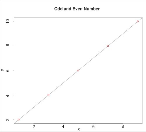
plot(y, x, col=”red”, main = “Odd and Even Numbers”, abline(lm(x~y)))
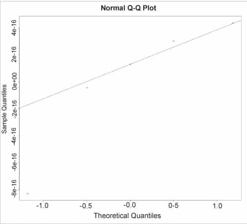
The normal QQ plot for the residual values can be displayed using the qqnorm() and qqline() functions, as shown below:
> qqnorm(r$resid)
> qqline(r$resid)
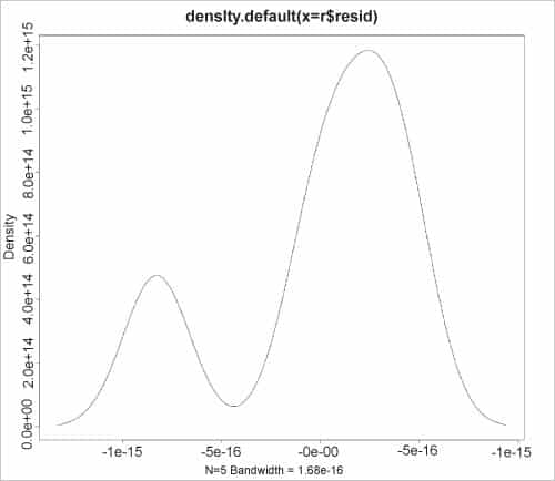
The kernel density estimates on the residuals can also be graphed using the plot() function, as shown in the figure.
> plot(density(r$resid))
The ls() function on the relation lists the various components of the ‘r’ object. For example:
> ls(r)
[1] “assign”    “call”    “coefficients”  “df.residual”
[5] “effects”  “fitted.values” “model”         “qr”
[9] “rank”      “residuals”     “terms”         “xlevels”
The components are briefly described below:
| Component | Description |
| assign | integer vector for each column |
| effects | named numeric vector |
| rank | numeric rank of the model |
| call | the matched call |
| fitted.values | the fitted mean values |
| residuals | response – fitted values |
| coefficients | named vector of coefficients |
| model | model frame used |
| terms | the ‘terms’ object |
| df.residual | residual degrees of freedom |
| qr | QR decomposition |
| xlevels | levels of the factors used in fitting |
> r$coefficients
(Intercept)           x
          1           1

> r$assign
[1] 0 1

> r$effects
  (Intercept)             x
-1.341641e+01  6.324555e+00  0.000000e+00 -4.440892e-16 -8.881784e-16

> r$rank
[1] 2

> r$call
lm(formula = y ~ x)

> r$fitted.values
 1  2  3  4  5
 2  4  6  8 10

> r$residuals
            1             2             3             4             5
4.367205e-16 -8.275904e-16  3.027995e-16  1.302899e-16 -4.221962e-17

> r$model
   y x
1  2 1
2  4 3
3  6 5
4  8 7
5 10 9

> r$terms
y ~ x
attr(,”variables”)
list(y, x)
attr(,”factors”)
  x
y 0
x 1
attr(,”term.labels”)
[1] “x”
attr(,”order”)
[1] 1
attr(,”intercept”)
[1] 1
attr(,”response”)
[1] 1
attr(,”.Environment”)
<environment: R_GlobalEnv>
attr(,”predvars”)
list(y, x)
attr(,”dataClasses”)
        y         x
“numeric” “numeric”

> r$df.residual
[1] 3

> r$qr
$qr
  (Intercept)           x
1  -2.2360680 -11.1803399
2   0.4472136   6.3245553
3   0.4472136  -0.1954395
4   0.4472136  -0.5116673
5   0.4472136  -0.8278950
attr(,”assign”)
[1] 0 1

$qraux
[1] 1.447214 1.120788

$pivot
[1] 1 2

$tol
[1] 1e-07

$rank
[1] 2

attr(,”class”)
[1] “qr”

> r$xlevels
named list()
The confint() function computes the confidence intervals for the parameters in the fitted model. For example:
> confint(r)
            2.5 % 97.5 %
(Intercept)     1      1
x               1      1
The confint() function accepts the following arguments:
| Argument | Description |
| object | fitted model object |
| parm | vector of numbers or names for the parameters |
| level | confidence level required |
| … | additional arguments |
The analysis of variance tables for the fitted model can be obtained using the anova() function, as follows:
 anova(r)
Analysis of Variance Table

Response: y
          Df Sum Sq Mean Sq    F value    Pr(>F)
x          1     40      40 1.2169e+32 < 2.2e-16 ***
Residuals  3      0       0
---
Signif. codes: 0 ‘***’ 0.001 ‘**’ 0.01 ‘*’ 0.05 ‘.’ 0.1 ‘ ’ 1
Consider the mtcars data set available in the lattice library:
> head(mtcars)
            mpg cyl disp  hp drat    wt  qsec vs am gear carb
Mazda RX4  21.0   6  160 110 3.90 2.620 16.46  0  1    4    4
Mazda RX4 Wag  21.0  6  160 110 3.90 2.875 17.02  0  1  4   4
Datsun 710   22.8   4  108  93 3.85 2.320 18.61  1  1  4    1
Hornet 4 Drive  21.4 6 258 110 3.08 3.215 19.44  1  0  3   1
Hornet Sportabout 18.7 8  360 175 3.15 3.440 17.02  0  0 3  2
Valiant    18.1   6  225 105 2.76 3.460 20.22  1  0    3    1
We can fit a regression between the number of cylinders and horsepower using the lm() function, as follows:
> m <- lm(cyl~hp, data=mtcars)
> print(m)

Call:
lm(formula = cyl ~ hp, data = mtcars)

Coefficients:
(Intercept)           hp
    3.00680      0.02168
A summary of the fitted model is shown below:
> summary(m)

Call:
lm(formula = cyl ~ hp, data = mtcars)

Residuals:
     Min       1Q   Median       3Q      Max
-2.27078 -0.74879 -0.06417  0.63512  1.74067

Coefficients:
            Estimate Std. Error t value Pr(>|t|)
(Intercept) 3.006795   0.425485   7.067 7.41e-08 ***
hp          0.021684   0.002635   8.229 3.48e-09 ***
---
Signif. codes:  0 ‘***’ 0.001 ‘**’ 0.01 ‘*’ 0.05 ‘.’ 0.1 ‘ ’ 1

Residual standard error: 1.006 on 30 degrees of freedom
Multiple R-squared:  0.693,	Adjusted R-squared:  0.6827
F-statistic: 67.71 on 1 and 30 DF,  p-value: 3.478e-09
Some of the individual components from the fitted model are listed below for reference:
> m$residuals
  Mazda RX4     Mazda RX4 Wag    Datsun 710    Hornet 4 Drive
 0.608014994   0.608014994    -1.023364771        0.608014994
 Hornet Sportabout   Valiant    Duster 360         Merc 240D
1.198584681    0.716432710     -0.319263348      -0.351174929
  ...

> m$model
                    cyl  hp
Mazda RX4             6 110
Mazda RX4 Wag         6 110
Datsun 710            4  93
Hornet 4 Drive        6 110
Hornet Sportabout     8 175

> m$terms
cyl ~ hp
attr(,”variables”)
list(cyl, hp)
attr(,”factors”)
    hp
cyl  0
hp   1
attr(,”term.labels”)
[1] “hp”
attr(,”order”)
[1] 1
attr(,”intercept”)
[1] 1
attr(,”response”)
[1] 1
attr(,”.Environment”)
<environment: R_GlobalEnv>
attr(,”predvars”)
list(cyl, hp)
attr(,”dataClasses”)
      cyl        hp
“numeric” “numeric”

> m$qr
$qr
                    (Intercept)            hp
Mazda RX4            -5.6568542 -829.78980772
Mazda RX4 Wag         0.1767767  381.74189579
Datsun 710            0.1767767    0.12620114
Hornet 4 Drive        0.1767767    0.08166844
Hornet Sportabout     0.1767767   -0.08860368
...

> confint(m)
                 2.5 %     97.5 %
(Intercept) 2.13783849 3.87575200
hp          0.01630186 0.02706522

> anova(m)
Analysis of Variance Table

Response: cyl
          Df Sum Sq Mean Sq F value    Pr(>F)
hp         1 68.517  68.517   67.71 3.478e-09 ***
Residuals 30 30.358   1.012
---
Signif. codes:  0 ‘***’ 0.001 ‘**’ 0.01 ‘*’ 0.05 ‘.’ 0.1 ‘ ’ 1
We can again use the predict() function to determine the number of cylinders required for a given horsepower. In the following example, we observe that in order to achieve 200 horsepower, we require at least 7 cylinders.
> hp <- data.frame(hp = 200)
> cyl <- predict(m, hp)
> cyl
       1
7.343504
You are encouraged to read the manual pages for the above R functions to learn more on their arguments, options and usage.


