

In the previous article in this series, we discussed the history of AI. We have also discussed matrices in detail earlier. In this third article in the series on AI, we will discuss more matrix operations. We will also get familiar with a few more Python libraries useful for developing AI.
Before we proceed any further, let us discuss a few significant terms often associated with AI and machine learning. Artificial neural networks (often called neural networks or NNs) are the core of machine learning and deep learning. But, what are they? By definition, they are computing models inspired by the biological neural networks that form human brains. I won’t be including the image of an NN here because the Internet nowadays is so full of it. But any person interested in AI has definitely seen one or more of those images, with an input layer on the left, one or more hidden layers in the middle, and an output layer on the right of the image. One important thing to understand is that the weights of edges between each layer, shown in the images we mentioned just now, keep on changing with training. This leads to successful machine learning and deep learning applications.
Supervised learning and unsupervised learning are two important models of machine learning. In the long run, any aspirant who wants to work in the field of AI or machine learning needs to learn about these models and the different techniques used to implement them. Hence, I think it is time for us to (informally) understand the difference between these two models. Consider two people named A and B who are supposed to classify apples and oranges into two separate groups. They have never seen apples or oranges. Both are given 100 photos of apples and oranges. But A has the additional information as to which are apples and which are oranges in the given photos. A is like a supervised algorithm. B does not have any additional information. All he/she has is the 100 photos. B is like an unsupervised algorithm. One day both start the classifications. Who will be better at his/her job? Conventional wisdom says A will outperform B. But machine learning says this may not be the case all the time. What if, out of the 100 images given to A, only 5 are of apples and the rest are all of oranges? He/she may not get familiar with apples at all. What if somebody intentionally cheated A by changing some of the labels of the photos, from apples to oranges and vice versa? In these scenarios, B could outperform A in the job.
But can this happen in a machine learning application for real? Yes! Imagine a situation where you are training your model with an inadequate or corrupted data set. This is just one of the many reasons why both these learning models, supervised and unsupervised, are still thriving in the fields of AI and machine learning. In the coming articles in this series, we will treat these topics more formally. Now let us learn to use JupyterLab, a very powerful tool available for developing AI based applications.
Introduction to JupyterLab
In the previous articles in this series, we were using the Linux terminal to run Python code for simplicity. Now, it is time to introduce yet another powerful player in the world of AI, JupyterLab. Remember, in the first article in this series we considered a few other alternatives to JupyterLab. But after considering various pros and cons of each and every one of them, we have decided to stick with JupyterLab. As JupyterLab is more powerful than Jupyter Notebook, our choice is further justified. There are many reasons for preferring JupyterLab over the Linux terminal while developing AI based applications. For example, the library and packages we need to use are often available by default in JupyterLab. Another reason is the ease of collaboration with a group of programmers or researchers. There are many other reasons too, and we will explore these in due course.
We have already learned how to install JupyterLab in the first article in this series. Assuming you have installed JupyterLab in your system, with the instructions given earlier, use the command jupyter lab or jupyter-lab to open JupyterLab in your default browser, like Mozilla Firefox, Google Chrome, etc. Figure 1 shows the launcher of the JupyterLab (just a part of the window) opened in my default browser. A Python shell called IPython (Interactive Python) is used in JupyterLab. But IPython has an independent existence and can be executed from your Linux terminal with the command ipython.
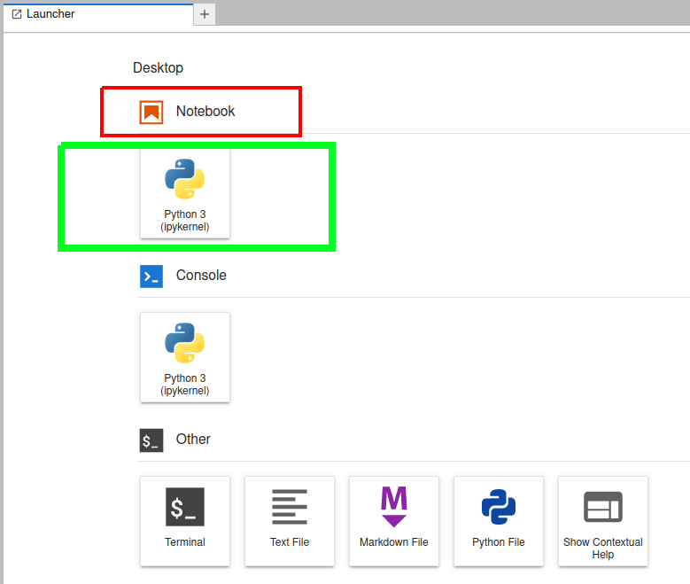
For the time being, we will start learning JupyterLab by using Jupyter Notebook alone, just one of the many features available with JupyterLab. In Figure 1, the button to be clicked to open a Jupyter Notebook is marked with a green rectangle. On clicking this button, you may be asked to select the kernel. If you have followed the installation steps given in this series, the sole choice would be Python 3 (ipykernel). But note that you can install kernels for programming languages like C++, R, MATLAB, Julia, etc, and many more in JupyterLab. Indeed, the complete list is quite large and can be found at https://github.com/jupyter/jupyter/wiki/Jupyter-kernels.
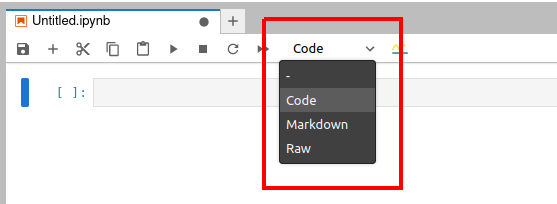
Now let us try to understand the working of a Jupyter Notebook very quickly. Figure 2 shows a Jupyter Notebook window. Notice that the extension of the open Jupyter Notebook file is .ipynb.
In Figure 2, you can see three different options, ‘code’, ‘markdown’, and ‘raw’ (marked with a red rectangle). These are the three types of cells you can use in a Jupyter Notebook. Code cells can be used for executable code. Markdown cells can be used for entering text data, and to write comments, explanations, etc. For example, if you are a computer trainer you can create interactive content of code and explanatory text, and share it with your students.
Unlike in a terminal, you can edit and rerun code in Jupyter Notebook, which is especially handy when you make simple typographical errors. Figure 3 shows how a few lines of Python code are executed in a Jupyter Notebook.
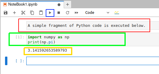
The button to execute the code in a cell is marked with a blue square. In order to execute the code in a cell, select that cell and then press this button. Figure 3 shows a markdown cell marked with a red rectangle, a code cell marked with a green rectangle, and the output of the code executed marked with a yellow rectangle. In this example, the Python code just prints the value of π (Pi).
As mentioned earlier, a number of libraries and packages are available in JupyterLab by default and you don’t need to install them in the beginning. You can import these libraries into your code by using the command import. The command !pip freeze will give you the complete list of libraries and packages currently available in your JupyterLab. If a library or package is not installed, then most of the time the command pip install package/library_name_in_all_lowercase_letters will work. For example, pip install tensorflow is the command to install the library TensorFlow in JupyterLab. I will explicitly mention the few times when there is a change in the installation command for a library. More powerful features of Jupyter Notebook and JupyterLab will be introduced as we proceed through this series.
Some complex matrix operations
Let us learn about a few more complex matrix operations. Consider the code given below. To save some space, I am not showing the output. I have added line numbers for convenience and they are not part of the code.
1. import numpy as np
2. A = np.arr ay([[1,2,3],[4,5,6],[7,8,88]])
3. B = np.arr ay([[1,2,3],[4,5,6],[4,5,6]])
4. print(A.T)
5. print(A.T.T)
6. print(np.trace(A))
7. print(np.linalg.det(A))
8. C=np.linalg.inv(A)
9. print(C)
10. print(A@C)
First, the package NumPy is imported in line 1. Then, two matrices A and B are created in lines 2 and 3. Line 4 prints the transpose of matrix A. Compare matrix A with the transpose of A to understand how the transpose operation works. Line 5 prints the transpose of the transpose of A. You will see that A and A.T.T are equivalent. This gives you another hint about the working of the operation transpose. Line 6 prints the trace of matrix A. The value printed will be 94, because trace is the sum of the diagonal (also called main diagonal) elements of matrix A. Notice that the main diagonal elements of A are 1, 5, and 88. Line 7 prints the determinant of A. When you execute this code, you will see that the answer is -237.00000000000009 (the value may change slightly in your machine). Since the determinant is non-zero, A is called a non-singular matrix. Line 8 stores the inverse of matrix A into matrix C. Line 9 prints matrix C. Line 10 prints the product of matrices A and C. On careful observation, you will see that the product is an identity matrix, a matrix where all the diagonal elements are 1 and all the other elements are 0. Note that exactly 1s and 0s will not be printed in the answer. For example, in the answer I got, there are numbers like -3.81639165e-17. Note that this is the scientific notation for a floating-point number, which is -3.81639165 × 10⁻¹⁷. This is -0.0000000000000000381639165, in decimal notation, which is very close to zero. Similarly, you can verify the other numbers in the answer.
On a side note, going through a tutorial on floating-point number representation in computers and the complications involved in it will definitely help you a lot and I highly recommend it. Now, by the convention adopted in the first article, we will try to classify between basic Python code and Python code for AI. In this case, all the lines of code, except lines 1 and 9, can be considered as code for AI.
Now apply lines 4 to 10 on matrix B. Lines 4 to 7 work as before. However, the determinant of B is 0 and hence it is called a singular matrix. Further, line 8 gives you an error because inverse exists only for non-singular matrices whose determinant is non-zero. Now, apply the same operations on all the eight matrices we have introduced in the previous article in this series. On seeing the outputs, you will get the additional insight that matrix operations like determinant and inverse are applicable only to square matrices.
Square matrices are matrices with an equal number of rows and columns. Though we tried to understand the working of these operations based on the above examples, I haven’t explained anything about the theory behind them. So, it would be a good idea to learn more about matrix operations like transpose, inverse, determinant, etc, if you have forgotten them. You could also learn about the different types of matrices like identity matrix, diagonal matrix, triangular matrix, symmetric matrix, skew symmetric matrix, etc. Wikipedia articles on these terms are a good starting point.
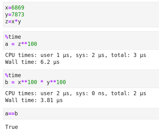
Now let us learn about some matrix operations that are even more complex, called matrix decomposition (also known as matrix factorization). First, let us recall integer factorization to understand the need for matrix factorization. The number 15 is the product of 3 and 5. But why do we need factorization? Consider the semi-prime (an integer which is the product of exactly two prime numbers) 54079637 whose factors are 6869 and 7873. I think the code and the output shown in Figure 4 give an answer to our question about the need for factorization. The line of code %time in the beginning shows us the time taken to execute a cell in Jupyter Notebook. Elementary number theory tells us that both the variables a and b contain the answer to the mathematical expression 54079637100. However, Figure 4 shows us that the answer in variable b is calculated much faster. Further, this reduction in execution time will become better and better as the number and the exponent in the above calculation increases.
Now let us move on to matrix decomposition. Similar to integer factorization, in matrix decomposition a matrix is written as the product of some other matrices. There are a lot of matrix decomposition techniques, and in almost all of them a matrix is written as the product of matrices that are more sparse than the original matrix. A sparse matrix is a matrix that has a lot of elements with value zero. Thus, after decomposition, we can work with sparse matrices rather than the original dense matrix with a lot of non-zero elements. In this article, we will discuss three decomposition techniques — LUP decomposition, eigendecomposition, and singular value decomposition (SVD).
But, in order to perform matrix decomposition, we need the services of yet another powerful Python library called SciPy. SciPy has functions for performing operations in linear algebra, integration, differentiation, optimisation, etc. In a sense, SciPy works on top of NumPy. First, let us discuss LUP decomposition. Any square matrix has an LUP decomposition. There is a variant of LUP decomposition called LU decomposition. However, not every square matrix has an LU decomposition. Hence, we discuss LUP decomposition.
In LUP decomposition, a matrix A is written as the product of three matrices L, U, and P. However, these three matrices do have some properties. L is a lower triangular matrix. A square matrix with all the entries above the main diagonal as zero is called a lower triangular matrix. U is an upper triangular matrix. A square matrix with all the entries below the main diagonal as zero is called an upper triangular matrix. P is a permutation matrix. This is a square matrix which has exactly one element with value 1 in each row and each column, and every other element of it has the value 0.
Now consider the code given below to perform LUP decomposition. Again, the line numbers have been added for convenience and are not part of the code.
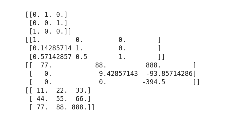
1. import numpy as np
2. import scipy as sp
3. A=np.rray([[11,22,33],[44,55,66],[77,88,888]])
4. P, L, U = sp.linalg.lu(A)
5. print(P)
6. print(L)
7. print(U)
8. print(P@L@U)
Figure 5 shows the output of the code. Lines 1 and 2 import packages NumPy and SciPy. A matrix A is created in line 3. Please keep in mind that we use matrix A throughout this section. Line 4 factorizes matrix A into three matrices — P, L, and U. Lines 5 to 7 print the matrices P, L, and U. From Figure 5, it is clear that P is a permutation matrix, L is a lower triangular matrix and U is an upper triangular matrix. Finally, line 10 multiplies the three matrices and prints the product matrix. Again, from Figure 5 it is clear that the product matrix P@L@U equals the original matrix A. Hence, the decomposition (factorization) property holds true. Further, you can verify from Figure 6 that matrices L, U, and P are more sparse (a lot of zero elements) than matrix A.
Now let us discuss eigendecomposition, in which a square matrix is represented in terms of its eigenvalues and eigenvectors. Though it is easy to calculate eigenvalues and eigenvectors using Python, a theoretical explanation about both is beyond the scope of our discussion. However, I encourage you to learn about these concepts (if you don’t know what they are already) so that you will have a clear idea about the actual operations you are performing. Again, the Wikipedia article on eigenvalues and eigenvectors is a good starting point. Now consider Figure 6, which shows the code for eigendecomposition.
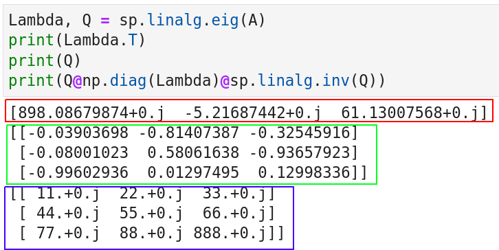
In Figure 6, line 1 finds the eigenvalues and eigenvectors. Lines 2 and 3 print them. Notice that a similar result can also be obtained with NumPy using the line of code Lambda, Q = np.linalg.eig(A). This also tells us that there is some overlap between NumPy and SciPy functions. Line 4 reconstructs the original matrix A. The code snippet np.diag(Lambda) in line 4 converts the eigenvalues into a diagonal matrix (we call it Λ). A diagonal matrix is a matrix in which all the elements outside the main diagonal are zero. The code snippet sp.linalg.inv(Q) in line 4 finds the inverse of Q (we call it Q-1). Finally, the three matrices Q, Λ, and Q-1 are multiplied together to obtain the original matrix A. Thus, in eigendecomposition A=QΛQ-1.
Figure 6 also shows the output of the code executed. The eigenvalues are marked with a red rectangle, the eigenvectors are marked with a green rectangle, and the reconstructed original matrix A is marked with a blue rectangle. But what are numbers like 11.+0.j doing in the output? Well, 11.+0.j is the complex number representation of the integer 11.
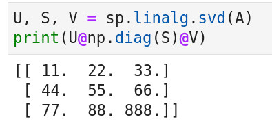
Let us now move on to singular value decomposition (SVD). It is a generalisation of eigendecomposition. Figure 7 shows the code and output of SVD. Line 1 decomposes matrix A into three matrices U, S, and V. In line 2, the code snippet ‘np.diag(S)’ converts S to a diagonal matrix. Finally, the three matrices are multiplied together to reconstruct the original matrix A. The advantage of SVD is that it can even diagonalize non-square matrices. However, the code for singular value decomposition of a non-square matrix is slightly more complicated and we won’t discuss it here for the time being.
A few more Python libraries for AI and machine learning
We now discuss two more libraries for developing AI and machine learning based applications. There is a reason why I didn’t say Python libraries. But we will come to that later. If you speak to a layperson about AI, what do you think will be the first image that will come to his/her mind? It will probably be a Terminator like scenario, where a machine can identify a person just by looking at him/her. Computer vision is one of the most important domains where AI and machine learning based applications are deployed a lot. So we are now going to get familiar with two libraries used in computer vision — OpenCV and Matplotlib. OpenCV (open source computer vision) is a library used mainly for real-time computer vision, and is developed using C and C++. C++ is the primary interface of OpenCV and that is the reason why I didn’t call it a Python library. However, Matplotlib is a plotting library for Python. One of my earlier articles in OSFY covers Matplotlib in a more detailed manner (https://www.opensourceforu.com/2018/05/scientific-graphics-visualisation-an-introduction-to-matplotlib).
There is an important reason for introducing these two libraries now. I have been preaching all this while that matrices are very important, but now I am going to give you a practical example of that. To illustrate this, let us read an image from our computer to a Jupyter Notebook, for further processing. We use Matplotlib for this task. Install Matplotlib with the command pip install matplotlib, if it is not available in your Jupyter Notebook. Figure 8 shows the code and the output that reads an image.
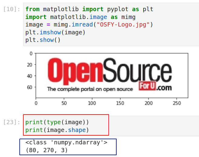
In the figure, lines 1 and 2 import some functions from Matplotlib. Notice that, if required, you can import individual functions or packages from a library instead of importing the whole library. These two lines contain basic Python code. Line 3 reads an image titled ‘OSFY-Logo.jpg’ from my computer. I have downloaded this image from the home page of the OSFY portal. This image is of height 80 pixels and width 270 pixels. Lines 4 and 5 display the image on a Jupyter Notebook window. But what is more important are the two lines of code shown below the image (marked with a red rectangle). The output of these lines of code tells us that the variable named image is actually a NumPy array. Further, it is a three-dimensional array of shape 80 x 270 x 3.
The two-dimensional array (80 x 270) part is clear from the size of the image mentioned earlier. But what about the third dimension? This is because of the fact that the image we saw is a colour image. Colour images in computers are often stored using the RGB colour model, where one layer is used for each of the three primary colours — red, green, and blue. I am sure all of you remember the experiments during our school days where primary colours were mixed to form different colours. For example, red and green when combined give yellow. The varying shades of each colour are often represented with numbers ranging from 0 (darkest) to 255 (brightest). Thus, a pixel with value (255, 255, 255) represents pure white colour.
Now, execute the command print(image). Parts of a large array will be shown in the Jupyter Notebook and you will see a lot of 255s printed in the beginning of the array. What is the reason for this? If you look at the logo of OSFY, you will understand the reason. There is a lot of white colour in the borders of the logo and hence a lot of 255s are printed in the beginning. On a side note, it is really informative to learn more about RGB colour models as well as other colour models like CMY, CMYK, HSV, etc.
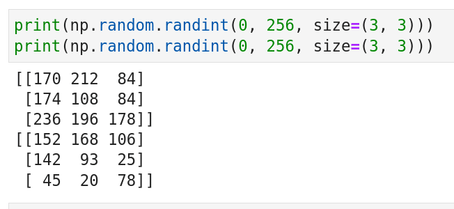
We now do the reverse process. We will create an image from an array. First, consider the code shown in Figure 9. It shows how two 3 x 3 matrices filled with random values between 0 and 255 are generated. Notice that though the same code is executed twice, the results are different. A pseudo-random number generator function of NumPy called randint does this. Indeed, the chances of my winning a lottery are far more than that of the two matrices being exactly equal.
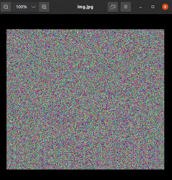
Our next plan is to generate a three-dimensional array of shape 512 x 512 x 3 and then convert it into an image. But for that we are going to use the library OpenCV. Be careful while installing OpenCV. The command for installing it is pip install opencv-python. Now consider the code shown below:
1. import cv2
2. img = np.random.randint(0, 256, size=(512, 512, 3))
3. cv2.imwrite(‘img.jpg’, img)
Line 1 imports the library OpenCV. Again, be careful, as the library name for the import statement is not opencv, unlike most other packages. Line 3 converts the matrix img to an image called img.jpg. Figure 10 shows this image generated by OpenCV. If you run this code in your system, the image will be generated in the same directory where your Jupyter Notebook is locally stored. If you check the properties of this image, you will see that it has a height of 512 pixels and width of 512 pixels. From these examples, it is easy to see that any AI or machine learning application that deals with computer vision uses a lot of arrays, vectors and matrices as well as ideas from linear algebra. Hence, our extensive treatment of arrays, vectors and matrices in this series is well justified.
Finally, consider the code shown below. What will the output image called image.jpg look like? I will give you two hints. The function zeros in lines 4 and 5 creates two 512 x 512 arrays green and blue filled with zeros. Lines 7 to 9 fill the three-dimensional array img1 with values from the arrays red, green, and blue.
1. import numpy as np
2. import cv2
3. red = np.random.randint(0, 256, size=(512, 512))
4. green = np.zeros([512, 512], dtype=np.uint8)
5. blue = np.zeros([512, 512], dtype=np.uint8)
6. img1 = np.zeros([512,512,3], dtype=np.uint8)
7. img1[:,:,0] = blue
8. img1[:,:,1] = green
9. img1[:,:,2] = red
10. cv2.imwrite(‘image.jpg’, img1)
We will wind up our discussion for now. In the next article in this series, we will begin by briefly learning about tensors, followed by installing and using a very powerful library called TensorFlow. TensorFlow is a serious player in the world of AI and machine learning.
Afterwards, we will take a break from matrices, vectors, and linear algebra for a short while and start learning a probability theory. If linear algebra is the brain of AI then probability is its heart, or vice versa.


