


With PandasAI, you can turn complex queries into simple conversations, unlocking insights that reshape your approach to data analysis. Let’s see how…
Business users and data analysts can now become more productive at work than ever before, thanks to OpenAI’s ChatGPT artificial intelligence tool. This new technology’s capacity to facilitate the creation of SQL queries is a significant perk for business analysts. For years, business analysts have used SQL to query and analyse data. Learning and writing SQL is now easier than the conventional approach, thanks to the usage of AI technology, which can swiftly and automatically generate, edit, debug, and optimise SQL queries.
Python Pandas is an open source toolkit that gives data scientists and analysts the ability to manipulate and analyse data. In the preprocessing stage of machine learning and deep learning, the Pandas library is particularly popular. Now, with generative AI capabilities, the PandasAI module enables conversational data frame operation features for queries to the record set of a DataFrame.
Conversational query
PandasAI provides great strength to Pandas. A great amount of time is usually required to prepare a data set for final analysis. With the help of the PandasAI generative tool, it is possible to initiate the desired data analysis task on the raw data set with minimal preprocessing.
As PandasAI works with Pandas like a supplementary tool, one can apply generative tools on Panda’s DataFrames and get back resultant DataFrames. OpenAI’s PandasAI can engage in dialogue with a machine to get the desired results in DataFrame format without the need for writing lengthy queries or graphical Python codes.
Use of PandasAI: Installation and setup
The first task is to install PandasAI using the pip install command from the command line:
C:\mypython> pip install pandasai
Once installation is complete, the system is ready for action. Here, the Google Colab platform is used to demonstrate the role of PandasAI in data analysis. Start by calling https://colab.research.google.com/ and then import the necessary modules as shown here:
import pandas as pd
import numpy as np
from pandasai import PandasAI
from pandasai.llm.openai import OpenAI
To upload the required input CSV file from the local directory, write down these file uploading instructions:
from google.colab import files
uploaded = files.upload()
Once this command is executed, Python will request an input file. A CSV file named CRISAT-WB_Rice.csv has been uploaded in this instance. The file contains 364 record sets detailing rice production in various districts of West Bengal. Interested readers can download the file using the link provided at the end of the article.
Exploring data with PandasAI
After uploading the input CSV file, proceed to read the CSV file from memory:
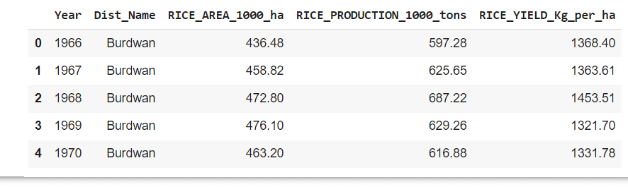
import pandas as pd
import io
df = pd.read_csv(io.StringIO(uploaded[‘ICRISAT-WB_Rice.csv’].decode(‘utf-8’)))

df.head()
The output is shown in Figure 1.
To call pandasai(), it is required to have a unique OpenAI API key. Obtain the key by creating an OpenAI account from https://openai.com/blog/chatgpt. From there it is possible to create an API key as shown here in Figure 2.
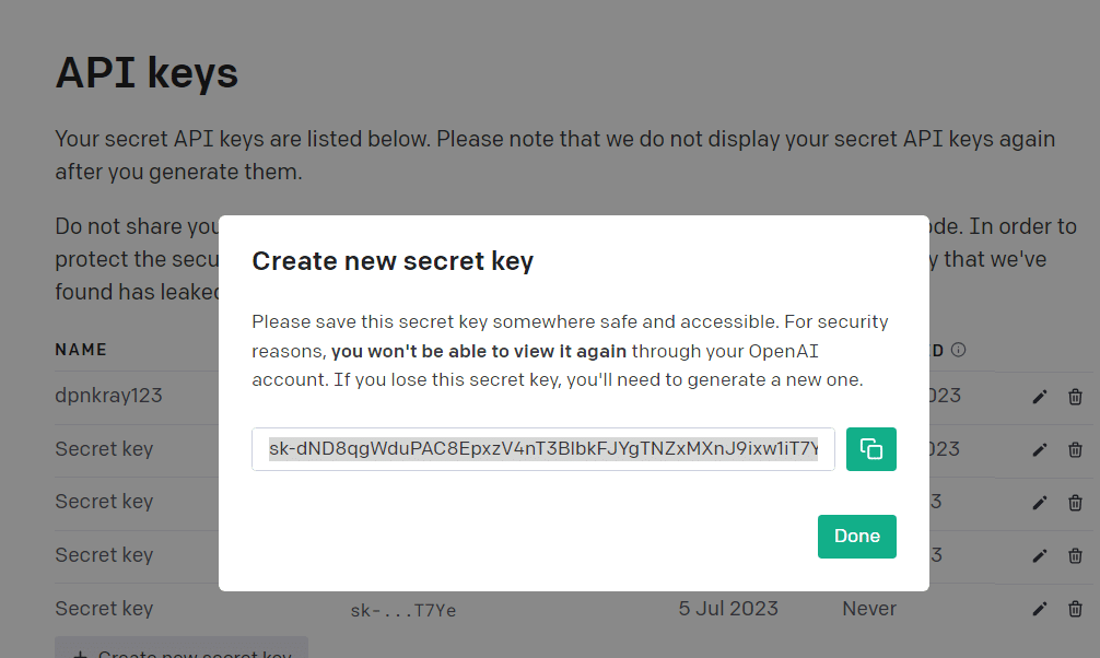
Once you have this key, you can call these two functions to start PandasAI:
oail = OpenAI(api_token=”Insert your API-KEY here”)
pandas_ai = PandasAI(oali, conversational=False)
For the ‘True’ value of the conversational option, PandasAI delivers a descriptive text record set, whereas it returns a tabular set of data sets for the ‘False’ value.
| Year | Dist_Name | RICE_AREA _1000_ha | RICE_PRODUCTION_ 1000_tons |
RICE YIELD Kg_per_ha |
| 1966 | Burdwan | 436.48 | 597.28 | 1368.4 |
| 1967 | Burdwan | 459.82 | 626.65 | 1364.61 |
| 1968 | Burdwan | 473.8 | 687.22 | 1454.51 |
| 1969 | Burdwan | 476.1 | 629.26 | 1322.7 |
| 1970 | Burdwan | 463.2 | 617.88 | 1332.78 |
| 1971 | Burdwan | 500.8 | 616.16 | 1233.81 |
| 1972 | Burdwan | 496 | 709.42 | 1430.28 |
| 1973 | Burdwan | 526.2 | 664.17 | 1262.2 |
| 1974 | Burdwan | 535.4 | 806.35 | 1506.07 |
Working with Pandas DataFrame
The index of a record can be explored with the pandas_ai() call:
# Finding the index of a row using the value of a column
result = pandas_ai(df, “What is the index of 1982?”)
print(result)
16
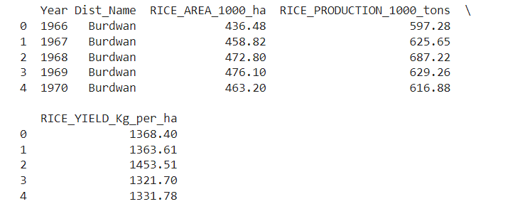
To display the first 5 records of the data set you can write this textual query:
response = pandas_ai(df, “Show 5 rows of data in tabular form”)
print(response)
The output is shown in Figure 3.
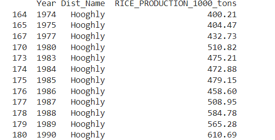
A more detailed conversational query can be written as follows:
response = pandas_ai(df, “Show 15 rows of data in tabular form   columns Year, DIST_NAME, RICE_PRODUCTION_1000_tons of DIST_NAME Hooghly RICE_PRODUCTION_1000_tons GREATER THAN 400”)
print(response)
The output is shown in Figure 4.
Similarly, we can also execute the following query over the DataFrame.
response = pandas_ai(df, “Show 15 rows of data in tabular form   columns Year, DIST_NAME and RICE_PRODUCTION_1000_tons DIST_NAME Bankura”)
print(response)
Data structure
It is possible to get all the basic structures of a DataFrame with simple textual instructions.
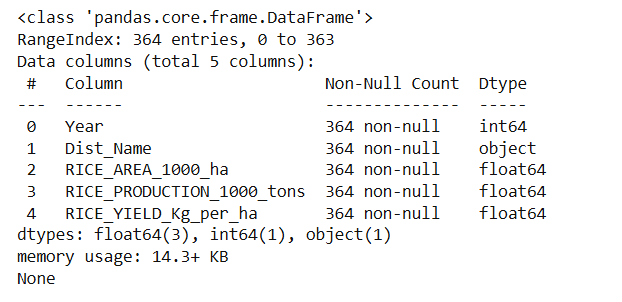
response = pandas_ai(df, “Show structure of data “)
print(response)
The shape of the DataFrame can also be explored with this instruction.
response = pandas_ai(df, “what is the shape of data?”)
print(response)
364 5
Data analysis
Overall basic statistics can easily be calculated with the following simple textual instruction:
response = pandas_ai(df, “what is the distribution  of RICE_PRODUCTION_1000_tans?”)
print(response)

count 364.000000
mean 641.068819
std 456.838868
min 51.490000
25% 289.392500
50% 493.310000
75% 848.247500
max 2145.290000
Name: RICE_PRODUCTION_1000_tons, dtype: float64
Skewness
To know the skewness of the distribution, you can use this simple query:
response = pandas_ai(df, “Show the skewness  of RICE_PRODUCTION_1000_tons”)
print(response)
1.2902333826377734
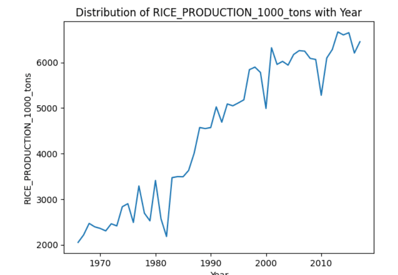
Graphics
Graphical representation is essential for effective data analysis. Distributions of different parameters can easily be plotted with the pandasai module with the help of ChatGPT. For example, the distribution of rice production can be depicted as follows:
response = pandas_ai(df, “Show the distribution graph  of RICE_PRODUCTION_1000_tons with Year”)
print(response)
Similarly, the distribution of rice production in a district can be plotted with an instruction like:
response = pandas_ai(df, “Show the distribution graph  of RICE_PRODUCTION_1000_tons with Year DIST_NAME Hooghly”)
print(response)
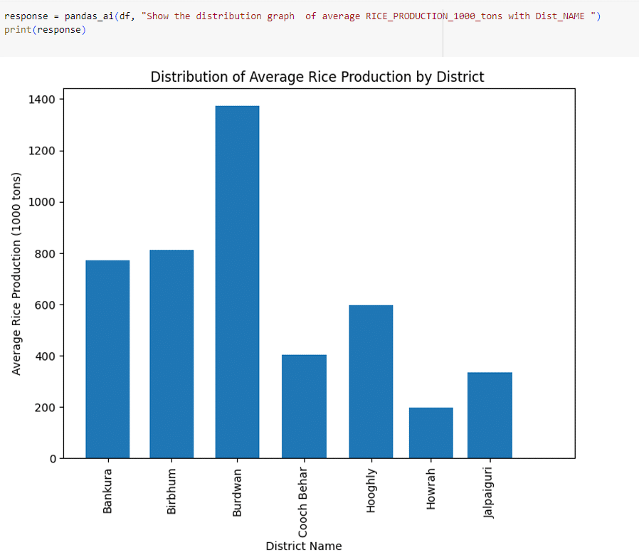
A bar graph of the district-wise distribution of rice production can easily be drawn with an instruction like this:
response = pandas_ai(df, “Show the distribution graph  of average RICE_PRODUCTION_1000_tons with Dist_NAME “)
print(response)
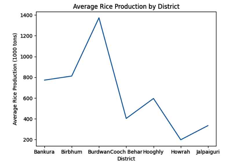
District-wise average rice production can be plotted like this:
df_sorted_rp=df.sort_values(by=’RICE_PRODUCTION_1000_tons’)

response = pandas_ai(df_sorted_rp, “line plot average RICE_PRODUCTION_1000_tons with DIST_NAME”)
print(response)
PandasAI, a supplementary tool based on ChatGPT, enhances data analysis in the Pandas environment. Its unstructured query language support makes data set analysis easier. Due to this textual informal approach, it is a paradigm change in data exploration and subsequent analysis. Here, we have focused on a few examples of the application of PandasAI on a data set. Readers can explore the several possibilities of this textual query-based data analysis. Programs and the data set are available at https://drive.google.com/drive/folders/1gVvRcwDNDP4j_RbYdBm7Z0FKcUp95wNQ?usp=sharing. Interested readers can download the data and explore it further.


