


In this 25th article in the ‘R, Statistics and Machine Learning’ series, we explore the caret package, which is a framework for building machine learning models in R.
The caret package provides miscellaneous functions for training classification and regression models. It allows you to tune parameters, use resampling techniques and make predictions from the models.
We will use R version 4.2.2 installed on Parabola GNU/Linux-libre (x86-64) for the R code snippets.
$ R --version

R version 4.2.2 (2022-10-31) -- “Innocent and Trusting”
Copyright (C) 2022 The R Foundation for Statistical Computing
Platform: x86_64-pc-linux-gnu (64-bit)

R is free software and comes with ABSOLUTELY NO WARRANTY.
You are welcome to redistribute it under the terms of the
GNU General Public License versions 2 or 3.

For more information about these matters, see https://www.gnu.org/licenses/.
Package installation
You can install and load the caret package using the following commands:
> install.packages(“caret”)

Installing package into ‘/home/shakthi/R/x86_64-pc-linux-gnu-library/4.1’
...

 * building package indices
 * installing vignettes
 * testing if installed package can be loaded from temporary location
 * checking absolute paths in shared objects and dynamic libraries
 * testing if installed package can be loaded from final location
 * testing if installed package keeps a record of temporary installation path
 DONE (caret)

> library(caret)
Loading required package: ggplot2
Loading required package: lattice
We will install and use a few additional packages to demonstrate the use of the caret package. The earth package implements multivariate adaptive regression splines (MARS). You can install and load this library using the following commands:
> install.packages(“earth”)
Installing package into ‘/home/shakthi/R/x86_64-pc-linux-gnu-library/4.1’
...

* building package indices
* testing if installed package can be loaded from temporary location
* checking absolute paths in shared objects and dynamic libraries
* testing if installed package can be loaded from final location
* testing if installed package keeps a record of temporary installation path

DONE (earth)

> library(earth)

Loading required package: Formula
Loading required package: plotmo
Loading required package: plotrix
Loading required package: TeachingDemos
The mda package provides mixture and flexible discriminant analysis, MARS, and vector-response smoothing splines. You can install and load the mda library using the following commands:
> install.packages(“mda”)

Installing package into ‘/home/shakthi/R/x86_64-pc-linux-gnu-library/4.1’
...
 ** checking absolute paths in shared objects and dynamic libraries
 * testing if installed package can be loaded from final location
 * testing if installed package keeps a record of temporary installation path
 DONE (mda)

> library(mda)
Loading required package: class
Loaded mda 0.5-4
Glass data set
The mlbench package contains numerous machine learning benchmark problems and data sets from the UCI repository. Let us use the Glass data set that contains 214 observations of chemical analysis of seven different types of glass.
> library(mlbench)
> data(Glass)
The set.seed() function is used to reset the random number generation. You can then take a sample data from the Glass data set for training and test validation as shown below:
> set.seed(103)
> train <- sample(1:dim(Glass)[1], 150)
> data <- Glass[ train, ]
> test <- Glass[-train, ]
The structure of the Glass data is given below:
> str(data)
‘data.frame’:	150 obs. of  10 variables:
 $ RI  : num  1.52 1.52 1.52 1.52 1.52 ...
 $ Na  : num  13.6 13.7 13.1 13.4 13.7 ...
 $ Mg  : num  3.87 3.84 3.45 3.49 0 3.5 3.26 3.61 0 3.48 ...
 $ Al  : num  1.27 0.72 1.76 1.52 0.56 1.48 2.22 1.54 3.04 1.35 ...
 $ Si  : num  72 71.8 72.5 72.7 74.5 ...
 $ K   : num  0.54 0.17 0.6 0.67 0 0.6 1.46 0.66 6.21 0.64 ...
 $ Ca  : num  8.32 9.74 8.38 8.08 10.99 ...
 $ Ba  : num  0 0 0 0 0 0 1.63 0 0 0 ...
 $ Fe  : num  0.32 0 0.17 0.1 0 0 0 0 0 0 ...
 $ Type: Factor w/ 6 levels “1”,”2”,”3”,”5”,..: 2 1 3 2 2 2 6 2 4 1 ...
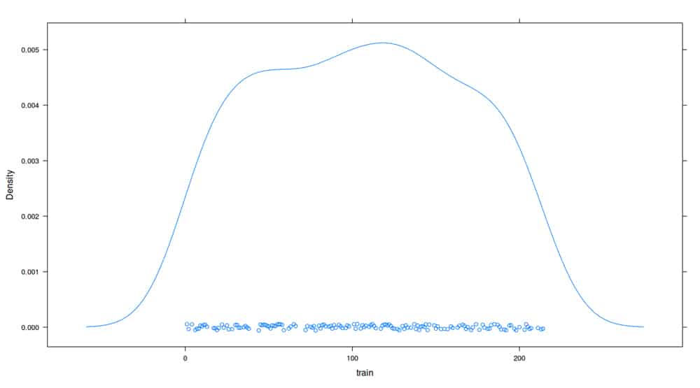
The densityplot() of the training data set is shown in Figure 1.
bagFDA()
The bagFDA() function is a wrapper function that uses multivariate adaptive regression splines (MARS) to implement flexible discriminant analysis (FDA). It accepts the following arguments:
| Argument | Description |
| x | A data frame or matrix of examples |
| y | A matrix or data frame of outcomes |
| weights | Weights for examples (Default: 1) |
| B | Number of bootstrap samples |
| keepX | Boolean to retain original training data |
| formula | Represented as y ~ x1 + x2 + … |
| data | Data frame from which variables are fetched |
| subset | An index vector listing the samples to be used |
| na.action | A function to be applied if data has NA |
> set.seed(501)
> fit <- bagFDA(Type ~ ., data)
predict()
The predict() function can classify observations with mda, and the data can be transformed into a matrix using the confusionMatrix() function as illustrated below:
> confusionMatrix(data = predict(fit, test[, -10]), reference = test[, 10])
Confusion Matrix and Statistics

          Reference
Prediction  1  2  3  5  6  7
         1 20  6  6  0  0  0
         2  2  9  2  2  0  0
         3  0  0  0  0  0  0
         5  0  1  0  2  0  1
         6  0  0  0  0  3  0
         7  0  0  0  0  0 10

Overall Statistics

               Accuracy : 0.6875
                 95% CI : (0.5594, 0.7976)
    No Information Rate : 0.3438
    P-Value [Acc > NIR] : 2.194e-08

                  Kappa : 0.5757

 Mcnemar’s Test P-Value : NA

Statistics by Class:

Class: 1 Class: 2 Class: 3 Class: 5 Class: 6 Class: 7
Sensitivity  0.9091  0.5625  0.000  0.50000  1.00000   0.9091
Specificity   0.7143  0.8750  1.000  0.96667  1.00000   1.0000
Pos Pred Value  0.6250  0.6000  NaN  0.50000 1.00000   1.0000
Neg Pred Value  0.9375  0.8571  0.875 0.96667 1.00000  0.9815
Prevalence  0.3438   0.2500   0.125  0.06250  0.04688  0.1719
Detection Rate  0.3125  0.1406  0.000 0.03125 0.04688  0.1562
Detection Prevalence 0.5000  0.2344  0.000  0.06250  0.04688   0.1562
Balanced Accuracy  0.8117 0.7188  0.500  0.73333  1.00000   0.9545
skim()
The skimr package provides summary statistics for a data set based on the principles of least surprise. You can install and load the library package as follows:
> install.packages(“skimr”)
Installing package into ‘/home/shakthi/R/x86_64-pc-linux-gnu-library/4.1’
...

 * testing if installed package can be loaded from temporary location
 * testing if installed package can be loaded from final location
 * testing if installed package keeps a record of temporary installation path
 DONE (skimr)

> library(skimr)
The skim() function gives a broad overview of the data frame. An example for the training data is given below:
> skimData <- skim(train)

> skimData
── Data Summary ────────────────────────────────
                           Values
Name                       train
Number of rows             150
Number of columns          1
_______________________
Column type frequency:
  numeric                  1
________________________
Group variables            None

── Variable type: numeric ────────────────────────────
  skim_variable n_missing complete_rate mean   sd p0  p25  p50  p75 p100 hist
1 data                  0             1 105. 60.7  1 53.2 106. 154.  214 ▇▇▇▇▆
downSample()
You can use the downSample() function to randomly obtain data from a set such that all the classes have the same frequency as the minor class. An example using the oil data set is illustrated below:
> data(oil)
> table(oilType)
oilType
 A  B  C  D  E  F  G
37 26  3  7 11 10  2

> downSample(fattyAcids, oilType)

   Palmitic Stearic Oleic Linoleic Linolenic Eicosanoic Eicosenoic Class
1     9.8   5.3  31.7   51.3    0.8   0.4    0.2     A
2     11.0  5.3  35.0   45.2    1.3   1.3    0.7     A
3     5.9   4.5  24.1   61.7    0.9   0.6    0.6     B
4     6.2   4.0  28.3   59.7    0.9   0.1    0.1     B
...
The downSample() function accepts the following arguments:
| Argument | Description |
| directory | A character vector of file path names |
| x | A matrix or data frame of variables |
| y | A factor variable |
| list | Boolean value to return a list or not |
| yname | A label for the class column |
upSample()
The upSample() function is similar to the downSample() function for the fatty acids data where additional samples are added to the minor class as shown below:
> upSample(fattyAcids, oilType)
    Palmitic Stearic Oleic Linoleic Linolenic Eicosanoic Eicosenoic Class
1    9.7   5.2  31.0     52.7     0.4     0.4      0.1     A
2    11.1  5.0  32.9     49.8     0.3     0.4      0.1     A
3    11.5  5.2  35.0     47.2     0.2     0.4      0.1     A
4    10.0  4.8  30.4     53.5     0.3     0.4      0.1     A
...
…You are encouraged to read the caret, mda and mlbench package reference manuals to learn more functions, arguments and their usage.


