























































In this fifth article in the series on quantum computing, we take a closer look at entanglement, meet the four Bell states, and examine the many ways in which a real superconducting quantum computer can go wrong.
In the previous article in this series (OSFY, September 2026), we finally left the comfortable world of the single qubit behind. We met the Controlled-NOT (CNOT) gate, our first multi-qubit gate, and used it to create a pair of entangled qubits. We also learned how to make Qiskit’s simulator misbehave on purpose by attaching a noise model to it, and we executed a quantum program on an actual superconducting quantum computer through the IBM Quantum Platform. At the end of that article, three promises were made: to look more deeply into entanglement, to introduce the Bell states, and to take a closer look at the various sources of error that affect today’s superconducting quantum computers. This article keeps all three promises.
The central theme of this article is quantum entanglement and, in particular, a family of four two-qubit states known as the Bell states. If superposition is what makes a single qubit interesting, entanglement is what makes a collection of qubits powerful. Erwin Schrödinger, who coined the term entanglement in 1935, went considerably further than that. He described it not as one interesting feature of quantum mechanics among many, but as the one feature that forces quantum mechanics to depart completely from classical ways of thinking. In the previous article we produced an entangled pair almost casually, with two lines of Qiskit code. In this article we shall find out what we actually produced.

As in the previous articles, we shall remain faithful to the three-level approach of this series and explore entanglement through code, mathematics and hardware. But before meeting the Bell states, let us honour a small tradition of this series: we shall first send our code to a real quantum computer.
Entanglement on real hardware
In the previous article, we executed the program qiskit8.py, a single-qubit Pauli-X circuit, on the IBM quantum processor ibm_marrakesh. That circuit involved just one qubit and one gate, and it was about as gentle a request as one can make of a quantum computer. Let us now raise the stakes. The program qiskit10.py, shown below, takes the two-qubit entangling circuit of qiskit9.py from the previous article—a Hadamard gate followed by a CNOT gate—and executes it on real superconducting hardware instead of the AerSimulator.
1. from qiskit import QuantumCircuit, transpile

2. from qiskit_ibm_runtime import QiskitRuntimeService, SamplerV2 as Sampler

3. API_KEY = “PasteYourAPIKeyHere”

4. QiskitRuntimeService.save_account(

channel=”ibm_quantum_platform”,

token=API_KEY,

set_as_default=True,

overwrite=True)

5. service = QiskitRuntimeService( )

6. backend = service.least_busy(operational=True,

simulator=False)

7. print(f”Running on backend: {backend.name}”)

8. qc = QuantumCircuit(2, 2)

9. qc.h(0)

10. qc.cx(0, 1)

11. qc.measure([0, 1], [0, 1])

12. transpiled_circuit = transpile(qc, backend)

13. sampler = Sampler(mode=backend)

14. job = sampler.run([transpiled_circuit], shots=1000)

15. print(“Job ID:”, job.job_id( ))

16. result = job.result( )

17. counts = result[0].data.c.get_counts( )

18. print(counts)
The program qiskit10.py is so close to qiskit8.py that a line-by-line explanation would waste space. Only three things are worth pointing out. First, the quantum part of the program—the four lines (8-11) that create two qubits, apply a Hadamard gate, apply a CNOT gate and measure both qubits—is character for character identical to qiskit9.py. Not a single line had to be changed to move from a simulator to a machine cooled to 15 millikelvin. That is a remarkable achievement of the Qiskit software stack, and it is worth pausing to admire it. Second, instead of the preset pass manager used in qiskit8.py, we simply call transpile( ) with the chosen backend as an argument. Both rewrite our circuit so that it uses only the operations the target processor physically supports—transpile( ) builds a preset pass manager internally—though it optimises a little harder, defaulting to level 2 where qiskit8.py asked for level 1. Third, save_account( ) writes the credentials to the file ~/.qiskit/qiskit-ibm.json, and set_as_default=True marks this account as the one to use when more than one has been saved. This is a one-time step: later programs can create a QiskitRuntimeService( ) object with no arguments and simply find the account.
A word of caution. Your API key is a password, not a decorative string. Never publish it, never commit it to a public repository, and never leave it in a screenshot. If one is ever exposed, revoke it on the IBM Quantum Platform and generate a new one.
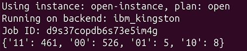
Before executing the program, activate the virtual environment with the command conda activate qiskit_env and make sure that the IBM Runtime package is installed, using pip install qiskit-ibm-runtime, exactly as we did in the previous article. Then replace the placeholder “PasteYourAPIKeyHere” with your own API key and run the command python qiskit10.py. The output obtained is shown in Figure 1.
IBM quantum processor
This time the least busy processor turned out to be ibm_kingston, a 156-qubit machine belonging to IBM’s Heron R2 family. The measurement statistics returned by the hardware are {‘11’: 461, ‘00’: 526, ‘01’: 5, ‘10’: 8}. Compare this with the ideal simulator output of the previous article, which contained nothing but 00 and 11. Here, 987 of the 1000 shots behaved themselves and produced the perfectly correlated outcomes we expect from the entangled state (|00+|11)/√2. The remaining 13 shots produced 01 or 10—outcomes that a perfectly entangled pair is simply not allowed to produce. Those 13 stray counts are the most interesting numbers in this article. On an ideal simulator, entanglement is a promise that is always kept; in this particular run, it was kept 98.7 per cent of the time. Let us now find out who broke the promise.
Where do the errors come from?
In the previous article we introduced the term Noisy Intermediate-Scale Quantum (NISQ) and noted that today’s processors are noisy. That is a little like saying that the monsoon is wet: true, but not very informative. A superconducting quantum computer fails in several distinct ways, each with its own physical origin, its own characteristic magnitude, and its own set of countermeasures. Let us look at the most important ones.
Energy relaxation, usually denoted T1, is the tendency of an excited qubit to give up its energy to the environment and fall back from |1 to |0. A qubit does not stay excited out of politeness; it stays excited only until the surrounding world persuades it otherwise. Both processors we have used—ibm_marrakesh in the previous article and ibm_kingston in this one—belong to IBM’s Heron family, where T1 is typically 100 to 300 microseconds, though the figure varies from qubit to qubit and from one calibration to the next. Notice that this error is not symmetric: a qubit decays from |1 to |0, but essentially never the other way round, because the refrigerator is far colder than the energy gap between the two levels.
Dephasing, denoted T2, is more subtle and, for readers of the third article in this series, more interesting. Here the qubit does not lose its energy; it loses its phase. Recall from the third article that a superposition carries a relative phase between |0 and |1, and that this phase, though invisible to a direct measurement, decides the outcome of every subsequent operation. Random fluctuations in the qubit’s frequency cause that phase to drift unpredictably, and once it has been randomised, the superposition has quietly degraded into an ordinary classical probability distribution. T2 is also typically in the range of 100 to 300 microseconds on Heron-class devices. Since a single-qubit gate takes only a few tens of nanoseconds, we have room for a few thousand operations before decoherence destroys the computation—which sounds generous until you recall that a useful quantum algorithm may need millions of operations.
Gate errors arise because the microwave pulses that implement our gates are not perfect. The pulse may be slightly too long, slightly off frequency, or slightly the wrong shape, so the state vector does not rotate through exactly the intended angle. On present-day Heron processors, single-qubit gates are extraordinarily good, with error rates of the order of a few parts in ten thousand. Two-qubit gates are roughly ten times worse, with error rates of a few parts in a thousand. That ten-to-one ratio shapes the whole of practical quantum programming. In the NISQ era, the number of two-qubit gates is the currency in which we pay for our algorithms, and circuit designers count them the way a jeweller counts grams. Our Bell circuit spends exactly one, which is why it came back so nearly intact.
Readout errors, also called measurement errors, occur at the very last step. The state of a superconducting qubit is read by bouncing a microwave signal off a resonator coupled to it and inspecting how the signal comes back. Occasionally the classification is simply wrong, and a qubit in |0 is reported as 1. Readout is usually the noisiest single operation on the chip, with error rates around one percent or a little below. Together with imperfect initialisation, these are known as SPAM errors—state preparation and measurement errors.
Crosstalk is the failure of qubits to mind their own business. Driving one qubit can disturb its neighbours, and two qubits that are physically adjacent can retain a small unwanted interaction even when we are not using it. This is precisely the problem that the tunable couplers of the Heron architecture were designed to solve: when a coupler is not needed, it is detuned so that the residual interaction is suppressed.
Leakage is a reminder that our tidy two-level picture is a convenient fiction. A transmon qubit (a type of superconducting charge qubit) is really an oscillator with many energy levels, of which we have borrowed the lowest two and named them |0 and |1. A badly shaped pulse can push the device into the second excited state, outside the computational space altogether. Such a qubit has not merely made an error—it has left the game.
Finally, there are the material and environmental villains. Microscopic defects in the oxide layers of the chip, known as two-level systems or TLS defects, drift in and out of resonance with the qubits and steal energy from them; the Heron R2 generation includes dedicated TLS mitigation for exactly this reason. And, spectacularly, cosmic rays occasionally strike the substrate and produce bursts of correlated errors across many qubits at once. It is a humbling thought that a quantum processor in a laboratory in the United States can be disturbed by a particle that began its journey outside the solar system
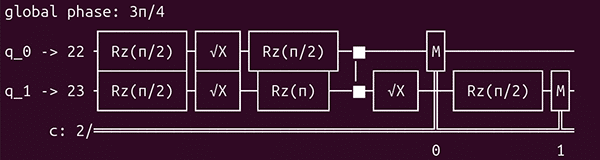
At this point, it is worth revealing something that the three-level approach of this series obliges us to confront. The CNOT gate we wrote in qiskit10.py does not exist on the chip. The Heron processor implements only a small set of native operations: the single-qubit gates X, SX (the square root of X) and RZ, and the two-qubit CZ (controlled-Z) gate. When transpile( ) prepares our circuit for the backend, our elegant Hadamard-plus-CNOT pair is rewritten as a sequence of RZ and SX rotations surrounding a single CZ gate. Try adding the statement print(transpiled_circuit.draw( )) to the program and see for yourself. The result is shown in Figure 2, and every gate in it is drawn from that short native list. Every physical error we have just discussed attaches itself to those operations, not to the idealised gates we wrote. Figure 2 also shows something the drawing of the original circuit could not: the labels q_0 -> 22 and q_1 -> 23 record which physical qubits on the 156-qubit chip the transpiler chose for us. Here we were fortunate, because qubits 22 and 23 are already neighbours on the lattice. Had they not been, the transpiler would have had to insert SWAP operations to bring them together, and each SWAP costs three more CZ gates.
The four Bell states
We are now ready for the central idea of this article. In 1935, Albert Einstein, Boris Podolsky and Nathan Rosen argued that quantum mechanics might not provide a complete description of reality. Their argument concerned entangled correlations: measuring one particle could reveal something about a distant partner. Surely, they reasoned, the result must already have been encoded in the pair through hidden variables that quantum mechanics had omitted. For nearly thirty years, the Einstein-Podolsky-Rosen (EPR) paradox remained largely a conceptual and philosophical dispute. That changed in 1964, when the Northern Irish physicist John Stewart Bell showed that local hidden-variable theories and quantum mechanics make measurably different predictions. A philosophical argument had become an experiment. Alain Aspect, John Clauser, and Anton Zeilinger conducted increasingly sophisticated experiments that supported the quantum predictions, and in 2022 they shared the Nobel Prize in Physics. Regular readers of this series may by now expect a Nobel laureate in every paragraph. Bell, however, is the exception that proves the rule. He died in 1990, and since Nobel Prizes are not awarded posthumously, he never received the honour. Although Bell never received a Nobel Prize, his theorem paved the way for others to receive science’s highest honour and helped settle one of the great philosophical disputes of modern physics.
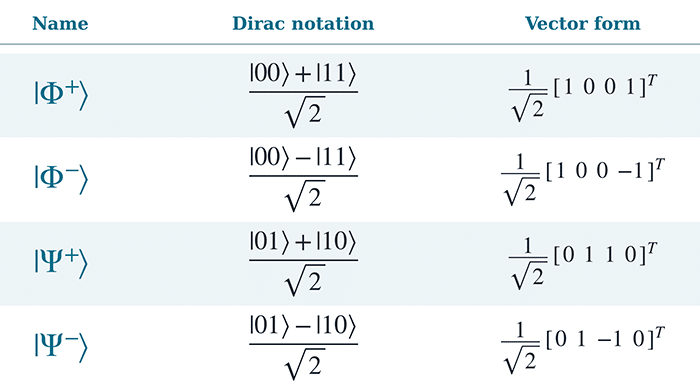
The four maximally entangled two-qubit states are named the Bell states in his honour. They are shown in Figure 3, written in the two notations this series has used since the first article: Dirac notation, the bra–ket notation named after the physicist and Nobel laureate Paul Dirac, and the vector form, which lists the four amplitudes in the order |00, |01, |10, |11, the superscript T marking the printed row as a column vector. Notice their structure: two of them, conventionally written |Φ+ and |Φ−, are superpositions of |00 and |11, and the other two, |Ψ+ and |Ψ−, are superpositions of |01 and |10. Within each pair, the two states differ only by a minus sign—which is to say, only by a phase. The state we have been producing since the previous article is |Φ+, obtained from |00 by a Hadamard gate followed by a CNOT gate.
Three properties make these four states special. First, they are maximally entangled: measuring either qubit alone yields 0 or 1 with equal probability, so an individual qubit of a Bell pair carries no information whatsoever, while the pair together is perfectly correlated. All the information lives in the relationship, not in the parts. Second, they are mutually orthogonal and form a complete basis for two qubits, called the Bell basis. Any two-qubit state can be written as a combination of these four, just as any single-qubit state can be written in terms of |0 and |1. Third—and this is the property we shall exploit shortly—all four can be reached from |Φ+ by operating on just one of the two qubits, leaving the other untouched.
Before we write any more code, a small but important warning about notation. Qiskit prints its bit strings with the highest-numbered qubit on the left. In a result such as ‘01’, the right-hand character is the outcome of qubit 0 (1 in this case) and the left-hand character is the outcome of qubit 1 (0 in this case). Until now nothing has depended on this. Our entangled results were 00 and 11, which read the same in either direction, and the stray 01 and 10 counts in Figure 1 were simply counted together as errors. From this point onwards, 01 and 10 are different answers and the ordering genuinely matters. This convention has confused more beginners than any quantum-mechanical subtlety, so it is worth committing to memory.
Now let us understand, at the mathematical level, what entanglement means. A two-qubit state is called separable, or unentangled, if it can be written as the product of two independent single-qubit states. Suppose |Φ+ = (|00+|11)/√2 were separable. Then we could write it as (α|0+β|1) (γ|0+δ|1), which expands to αγ|00+αδ|01+βγ|10+βδ|11. Comparing coefficients, we need αγ = 1/√2 and βδ = 1/√2, so none of the four numbers may be zero. But we also need αδ = 0 and βγ = 0, which forces at least one of them to be zero. The two requirements contradict each other, so no such factorisation exists. That short argument is the whole definition: an entangled state is one that cannot be described by describing its parts separately. There is no mysterious influence travelling between the qubits. There is simply no longer any such thing as ‘the state of qubit 0’.
Figure 3 tells us what the four states are, but not how to make them. All four begin with the same Hadamard and CNOT pair that produced |Φ+ in the previous article; what differs is the operation applied afterwards, and it acts on qubit 1 alone. Z turns |Φ+ into |Φ−, X turns it into |Ψ+, and X followed by Z turns it into |Ψ−. That is the third property above, expressed as a recipe: the four Bell states differ only by an operation on a single member of the pair.
Now look at what separates |Φ+ from |Φ−. It is a single minus sign, and by now that should be setting off an alarm bell. In the third article of this series we met exactly this situation with a single qubit: the Pauli-Z gate appeared to do nothing at all, because a phase cannot be seen in the measurement statistics. Does the same disappointment await us here?
Telling the Bell states apart
Let us find out. The program qiskit11.py, shown below, prepares all four Bell states in turn and measures each of them in the computational basis.
1. from qiskit import QuantumCircuit, transpile

2. from qiskit_aer import AerSimulator

3. bell_states = {“Phi+”: “”, “Phi-”: “Z”, “Psi+”: “X”, “Psi-”: “XZ”}

4. sim = AerSimulator( )

5. for name, local_gates in bell_states.items( ):

6. qc = QuantumCircuit(2, 2)

7. qc.h(0)

8. qc.cx(0, 1)

9. if “X” in local_gates:

10. qc.x(1)

11. if “Z” in local_gates:

12. qc.z(1)

13. qc.measure([0, 1], [0, 1])

14. compiled = transpile(qc, sim)

15. counts = sim.run(compiled, shots=1000).result( ).get_counts( )

16. print(name, counts)
Now let us understand how the program works. Line 3 defines a dictionary whose keys name the four Bell states and whose values record the extra gates each one needs. Line 5 loops over them. Lines 6 to 8 build the |Φ+ circuit we already know, and Lines 9 to 12 apply the extra gates to qubit 1. Line 13 measures both qubits, and Lines 14 to 16 run the circuit for 1000 shots and print the counts. Remember to activate qiskit_env before running the program.
The results are shown in Figure 4, and the outcome is disappointing in a very instructive way. Both |Φ+ and |Φ− produce roughly 500 counts of 00 and 500 of 11. Both |Ψ+ and |Ψ− produce roughly 500 counts of 01 and 500 of 10. Four distinct, mutually orthogonal quantum states have collapsed into two indistinguishable pairs of statistics. The reason is arithmetic: a probability is the squared magnitude of an amplitude, and both +1/√2 and −1/√2 square to the same 1/2. The minus sign is still in the state; it simply does not survive the squaring.
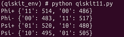
Two orthogonal quantum states—as different as two states can be, and distinguishable in principle with perfect certainty—have been made to look identical simply by asking the wrong question. The information is not missing. We are asking in the wrong language.
So let us ask properly. Recall from the second article that quantum gates are reversible. If the circuit H followed by CNOT turns |00 into |Φ+, then running that circuit backwards—CNOT followed by H—must turn |Φ+ back into |00. And since the four Bell states form a basis, the same reversed circuit should map each of the other three to a different computational basis state. This procedure is called a Bell measurement, and the program ‘qiskit12.py’, shown below, implements it.
1. from qiskit import QuantumCircuit, transpile

2. from qiskit_aer import AerSimulator

3. bell_states = {“Phi+”: “”, “Phi-”: “Z”, “Psi+”: “X”, “Psi-”: “XZ”}

4. sim = AerSimulator( )

5. for name, local_gates in bell_states.items( ):

6. qc = QuantumCircuit(2, 2)

7. qc.h(0)

8. qc.cx(0, 1)

9. if “X” in local_gates:

10. qc.x(1)

11. if “Z” in local_gates:

12. qc.z(1)

13. qc.cx(0, 1)

14. qc.h(0)

15. qc.measure([0, 1], [0, 1])

16. compiled = transpile(qc, sim)

17. counts = sim.run(compiled, shots=1000).result( ).get_counts( )

18. print(name, counts)
Now let us understand how the program works. The only new statements are Lines 13 and 14, which apply a CNOT gate and then a Hadamard gate before the measurement in Line 15. That is the preparation circuit of Lines 7 and 8, run in reverse order. Everything else is unchanged.
The output is shown in Figure 5, and it is one of the most satisfying results we have obtained in this series. The state |Φ+ yields ‘00’ in all 1000 shots. |Φ− yields ‘01’ in all 1000 shots. |Ψ+ yields ‘10’ every time, and |Ψ− yields ‘11’ every time. Not approximately, not on average—every single shot. The randomness has vanished completely, and the four states that were indistinguishable a moment ago are now labelled with perfect certainty.
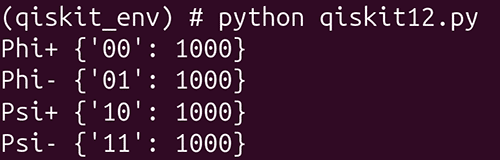
Take a moment to appreciate what has happened, because it contains the seed of everything that follows in this series. The phase difference between |Φ+ and |Φ− was invisible to measurement. By applying two more gates before measuring, we converted that invisible phase into a difference in outcomes that is not merely visible but absolutely certain. This is the same trick we used in the third article, when a second Hadamard gate exposed the hidden work of the Pauli-Z gate, and it has a name: quantum interference. Every quantum algorithm worth the name is, at bottom, an elaborate arrangement of this trick.
It is now time to conclude. In this article we executed an entangling circuit on a real 156-qubit superconducting processor and found 13 shots out of 1000 that had no business being there. Chasing those 13 counts took us through the whole zoo of errors that afflict present-day quantum hardware—relaxation, dephasing, gate errors, readout errors, crosstalk, leakage, material defects, and cosmic rays. We then met the four Bell states, proved what it means for a state to be entangled, discovered that measurement in the computational basis cannot tell all four apart, and repaired that failure with a Bell measurement.
That last experiment left us with a loose thread, and it is deliberately loose. Twice now we have made a hidden phase visible by applying an extra gate before measuring: once with a single qubit in the third article, and once with a Bell pair in this one. Both times the revealing gate was the Hadamard—the first gate we ever met, and the one we have used most often without examining it closely. In the next article we shall give the Hadamard operator the attention it deserves and then turn to the phenomenon it has quietly been exploiting all along: quantum interference. We shall see how the cancellation of unwanted amplitudes—not some fantasy of trying every answer at once—is the real engine of quantum speedup. Entanglement, it turns out, was only half the story.