What is Scientific Programming?

Scientific programming, or in broader terms, scientific computing, deals with solving scientific problems with the help of computers, so as to obtain results more quickly and accurately. Computers have long been used for solving complex scientific problems — however, advancements in computer science and hardware technologies over the years have also allowed students and academicians to play around with robust scientific computation tools.

Although tools like Mathematica and Matlab remain commercial, the open source community has also developed some equally powerful computational tools, which can be easily used by students and independent researchers. In fact, these tools are so robust that they are now also used at educational institutions and research labs across the globe.

So, let’s move on to setting up a scientific environment.

Setting up the environment

Most UNIX system/Linux distributions have Python installed by default. We will use Python 2.6.6 for the purposes of this article. It’s recommended to install IPython, as it offers enhanced introspection, additional shell syntax, syntax highlighting and tab-completion. You can install IPython here.

Next, we’ll install the two most basic scientific computational packages for Python: NumPy and SciPy. The former is the fundamental package needed for scientific computing with Python. It contains a powerful N-dimensional array object, sophisticated functions, tools for integrating C/C++, and Fortran code with useful linear algebra, Fourier transforms, and random-number capabilities. The SciPy library is built to work with NumPy arrays, and provides many user-friendly and efficient numerical routines for numerical integration and optimisation.

Open the Synaptic Package Manager and install the python-numpy and python-scipy packages. Now that we have NumPy and SciPy installed, let’s get our hands dirty with some mathematical functions and equations!

Numerical computations with NumPy, SciPy and Maxima

NumPy offers efficient array computations with fixed-size, homogeneous, multi-dimensional array types, and a plethora of functions to perform various array operations. Array-programming languages like NumPy generalise operations in scalars to apply transparently to vectors, matrices and other higher-dimensional arrays. Python does not have a default array data type, and processing data with Python lists and for loops is dramatically slower compared to corresponding operations in compiled languages like FORTRAN, C and C++. NumPy comes to the rescue, with its dynamically typed environment for array computation, similar to basic Matlab. You can create a simple array with the array function in NumPy:

In[1]: import numpy as np

In[2]:  a = np.array([1,2,3,4,5])

In[2]:  b = np.array([6,7,8,9,10])

In[3]:  type(b) #check datatype

Out[3]: type numpy.ndarray  #array

In[4]:  a+b

Out[4]: array([7,9,11,13,15])

You can also convert a simple array to a matrix array using the shape attribute.

In[1]: import numpy as np

In[5]:  c = np.array([1,4,5,7,2,6])

In[6]:  c.shape = (2,3)

In[7]:  c

Out[7]: array([1,4,5],[7,2,6]) // converted to a 2 column matrix

Matrix operations

Now let us take a look at some simple matrix operations. The following matrix can be simply defined as:
[latex]M = \begin{pmatrix}
1 & 2 & 3 \\
4 & 5 & 6 \\
7 & 8 & 9
\end{pmatrix}[/latex]

# Defining a matrix and matrix multiplication

In[1]: import numpy as np

In[2]: x = np.array([[1,2,3],[4,5,6],[7,8,9]])

In[3]: y = np.array([[1,4,5],[2,6,5],[6,8,3]]) #another matrix

In[4]: z = np.dot(x,y) #matrix multiplication using dot attribute

In[5]: z

Out[5]: z = ([[23, 40,24], [50,94,63],[77,148,102]])

You can also create matrices in NumPy using the matrix class. However, it’s preferable to use arrays, since most NumPy functions return arrays, and not matrices. Moreover, matrix objects have a maximum of Rank-2. To hold Rank-3 data, you need an array. Also, arrays are closer in semantics to tensor algebra,  compared to matrix objects.

The following example shows how to transpose a matrix and define a diagonal matrix:

In[7]: import numpy as np

In[8]: x = np.array([[1,2,3],[4,5,6],[7,8,9]])

In[7]: xT = np.transpose(x) #take transpose of the matrix

In[8]: xT

Out[8]:xT = ([[1,4,7],[2,5,8],[3,6,9]])


In[9]:n = diag(range(1,4)) #defining a diagnol matrix

In[10]: n

Out[10]:n = ([[1,0,0],[0,2,0],[0,0,3]])

Linear algebra

You can also solve linear algebra problems using the linalg package contained in SciPy. Let us look at a few more examples of calculating matrix inverse and determinant:

# Matrix Inverse 

In[1]: import numpy as np

In[2]:  m = np.array([[1,3,3],[1,4,3],[1,3,4]])

In[3]:  np.linalg.inv(m) #take inverse with linalg.inv function

Out[3]: array([[-7,-3,-3],[-1,1,0],[-1,0,1]])


#Calculating Determinant

In[4]:  z = np.array([[0,0],[0,1]])

In[5]:  np.linalg.det(z)

Out[5]: 0  #z is a singular matrix and hence has its determinant as zero

Integration

The scipy.integrate package provides several integration techniques, which can be used to solve simple and complex integrations. The package provides various methods to integrate functions. We will be discussing a few of them here. Let us first understand how to integrate the following functions:
[latex]\int_3^0 \! x^2 dx \\ \\
\int_3^1 \! 2^{\sqrt{x}} /\sqrt{x} dx[/latex]

# Simple Integration of x^2
 
In[1]: from scipy.integrate import quad
 
In[2]: import scipy as sp
 
In[3]: sp.integrate.quad(lambda x: x**2,0,3) 
 
Out[3]: (9.0, 9.9922072216264089e-14)
 
 
# Integration of 2^sqrt(x)/sqrt(x) 
 
In[4]: sp.integrate.quad(lambda x: 2**sqrt(x)/sqrt(x),1,3)
 
Out[4]: (3.8144772785946079, 4.2349205016052412e-14)

The first argument to quad is a “callable” Python object (i.e., a function, method, or class instance). We have used a lambda function as the argument in this case. (A lambda function is one that takes any number of arguments — including optional arguments — and returns the value of a single expression.) The next two arguments are the limits of integration. The return value is a tuple, with the first element holding the estimated value of the integral, and the second element holding an upper bound on the error.

Differentiation

We can get a derivative at a point via automatic differentiation, supported by FuncDesigner and OpenOpt, which are scientific packages based on SciPy. Note that automatic differentiation is different from symbolic and numerical differentiation. In symbolic differentiation, the function is differentiated as an expression, and is then evaluated at a point. Numerical differentiation makes use of the method of finite differences.

However, automatic differentiation is the decomposition of differentials provided by the chain rule. A complete understanding of automatic differentiation is beyond the scope of this article, so I’d recommend that interested readers refer to Wikipedia. Automatic differentiation works by decomposing the vector function into elementary sequences, which are then differentiated by a simple table lookup.

Unfortunately, a deeper understanding of automatic differentiation is required to make full use of the scientific packages provided in Python. Hence, in this article, we’ll focus on symbolic differentiation, which is easier to understand and implement. We’ll be using a powerful computer algebra system known as Maxima for symbolic differentiation.

Maxima is a version of the MIT-developed MACSYMA system, modified to run under CLISP. Written in Lisp, it allows differentiation, integration, solutions for linear or polynomial equations, factoring of polynomials, expansion of functions in the Laurent or Taylor series, computation of the Poisson series, matrix and tensor manipulations, and two- and three-dimensional graphics.

Open the Synaptic Package Manager and install the maxima package. Once installed, you can run it by executing the maxima command in the terminal. We’ll be differentiating the following simple functions with the help of Maxima:

d / dx(x⁴)
d / dx(sin x + tan x)
d / dx(1 / log x)

Figure 2 displays Maxima in action.

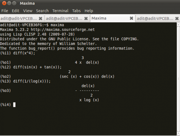
You have to simply define the function in diff() and maxima will calculate the derivative for you.

(%i1) diff(x^4)

(%o1) 4x^3 del(x)

(%i2) diff(sin(x) + tan(x))

(%o2) (sec^2(x) + cos(x))del(x)

(%i3) diff(1/log(x))

(%o3) - del(x)/x log^2(x)-

The command diff(expr,var,num) will differentiate the expression in Slot 1 with respect to the variable entered in Slot 2 a number of times, determined by a positive integer in Slot 3. Unless a dependency has been established, all parameters and variables in the expression are treated as constants when taking the derivative. Similarly, you can also calculate higher order differentials with Maxima.

Ordinary differential equations

Maxima can also be used to solve ODEs. We’ll dive straight into some examples to understand how to solve ODEs with Maxima. Consider the following differential equations:

dx/dt = e^-t + x
d²x / dt² – 4x = 0

Consider Figure 3.

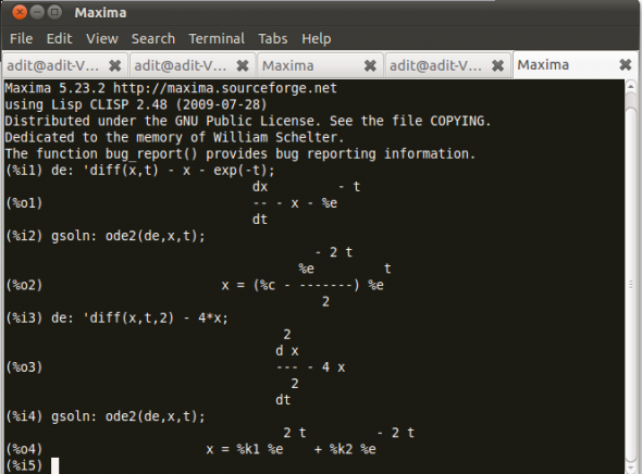
Let’s rewrite our example ordinary differential equations using the noun form diff, which uses a single quote. Then use ode2, and call the general solution gsoln.

The function ode2 solves an ordinary differential equation (ODE) of the first or second order. This takes three arguments: an ODE given by eqn, the dependent variable dvar, and the independent variable ivar. When successful, it returns either an explicit or implicit solution for the dependent variable. %c is used to represent the integration constant in the case of first-order equations, and %k1 and %k2 the constants for second-order equations.

We can also find the solution at predefined points using ic1 and call this particular solution, psoln. Consider the following non-linear first order differential equation:

(x²y)dy / dx = xy +x³ – 1

Let’s first define the equation, and then solve it with ode2. Further, let us find the particular solution at points x=1 and y=1 using ic1.

We can also solve ODEs with NumPy and SciPy using the FuncDesigner and OpenOpt packages. However, both these packages make use of automatic differentiation to solve ODEs. Hence, Maxima was chosen over these packages. ODEs can also be solved using the scipy.integrate.odeint package. We will later use this package for mathematical modelling.

Curve plotting with MatPlotLib

It’s said that a picture is worth a thousand words, and there’s no denying the fact that it’s much more convenient to make sense of a scientific experiment by looking at the plots as compared to looking just at the raw data.

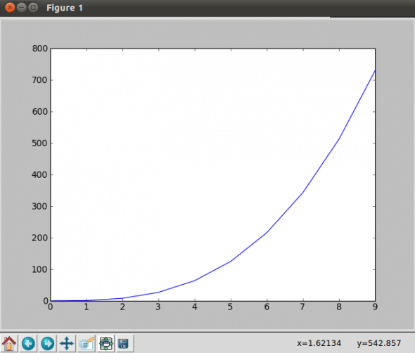
In this article, we’ll be focusing on MatPlotLib, which is a Python package for 2D plotting that produces production-quality graphs. Matlab is customisable and extensible, and is integrated with LaTeX markup, which is really useful when writing scientific papers. Let us make a simple plot with the help of MatPlotLib:

#Simple Plot with MatPlotLib

#! /usr/bin/python

import matplotlib.pyplot as plt

x = range(10)

plt.plot(x, [xi**3 for xi in x])

plt.show()

Let us take another example using the arange function; arange(x,y,z) is a part of NumPy, and it generates a sequence of elements with x to y with spacing z.

#Simple Plot with MatPlotLib

#! /usr/bin/python

import matplotlib.pyplot as plt
import numpy as np

x = np.arange(0,20,2)

plt.plot(x, [xi**2 for xi in x])

plt.show()

We can also add labels, legends, the grid and axis name in the plot. Take a look at Figure 6, and the following code:

import matplotlib.pyplot as plt
import numpy as np

x = np.arange(0,20,2)

plt.title('Sample Plot')

plt.xlabel('X axis')

plt.ylabel('Y axis')

plt.plot(x, [xi**3 for xi in x], label='Fast')

plt.plot(x, [xi**4 for xi in x], label='Slow')

plt.legend()

plt.grid(True)

plt.show()

plt.savefig('plot.png')

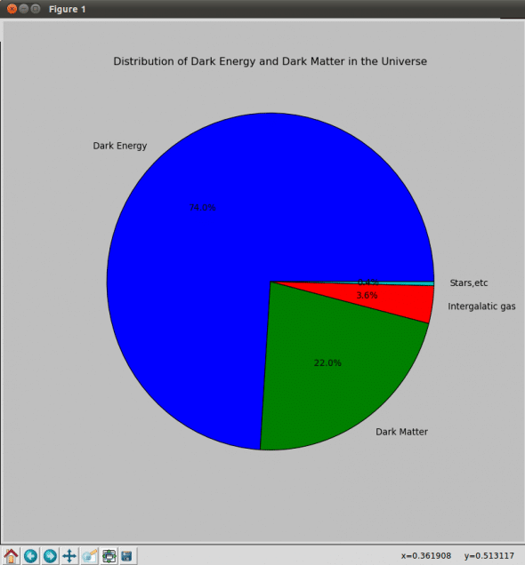
You can create various types of plots using MatPlotLib. Let us take a look at Pie Plot and Scatter Plot.

import matplotlib.pyplot as plt

plt.figure(figsize=(10,10));

plt.title('Distribution of Dark Energy and Dark Matter in the Universe')

x = [74.0,22.0,3.6,0.4]

labels = ['Dark Energy', 'Dark Matter', 'Intergalatic gas', 'Stars,etc']

plt.pie(x, labels=labels, autopct='%1.1f%%');

plt.show()

import matplotlib.pyplot as plt

import numpy as np

plt.title('Scatter Plot')

x = np.random.randn(200)

y = np.random.randn(200)

plt.xlabel('X axis')

plt.ylabel('Y axis')

plt.scatter(x,y)

plt.show()

Similarly, you can plot Histograms and Bar charts using the plt.hist() and plt.bar() functions, respectively. In our next example, we will generate a plot by using data from a text file:

import matplotlib.pyplot as plt 
import numpy as np

data = np.loadtxt('ndata.txt') 
x = data[:,0] 
y = data[:,1] 

figure(1,figsize=(6,4))

grid(True) 
hold(True) 
lw=1

xlabel('x') 

plot(x,y,'b',linewidth=lw) 

plt.show()

After executing this program, it results in the plot shown in Figure 10.

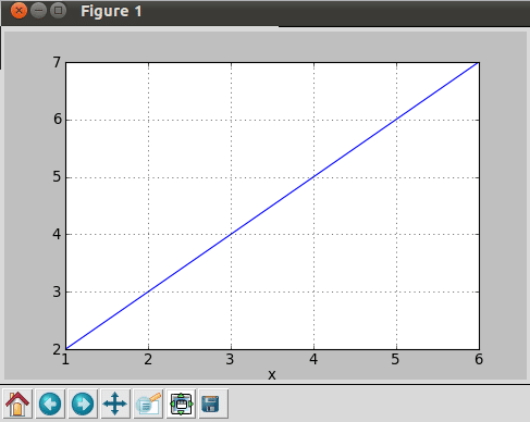
So, what’s happening here? First of all, we fetch data from the text file using the loadtxt function, which splits each non-empty line into a sequence of strings. Empty or commented lines are just skipped. The fetched data is then distributed in variables using slice. The figure function creates a new figure of the specified dimensions, whereas the plot function creates a new line plot.

Mathematical modelling

Now that we have a basic understanding of various computation tools, we can move on to some more complex problems related to mathematics and physics. Let’s take a look at one of the problems provided by the SciPy community. The example is available on the Internet (at the SciPy website). However, some of the methods explained in this example are deprecated; hence, we’ll rebuild the example, so that it works correctly with the latest version of SciPy and NumPy.

We’re going to build and simulate a model based on a coupled spring-mass system, which is essentially a harmonic oscillator, in which a spring is stretched or compressed by a mass, thereby developing a restoring force in the spring, which results in harmonic motions when the mass is displaced from its equilibrium position. For an undamped system, the motion of Block 1 is given by the following differential equation:

m₁d²x₁ / dt = (k₁ + k)x₁ – k₂x₂ = 0

For Block 2:

m₂d²x₂ / dt + k x₂ – k₁x₁ = 0

In this example, we’ve taken a coupled spring-mass system, which is subjected to a frictional force, thereby resulting in damping. Note that damping tends to reduce the amplitude of oscillations in an oscillatory system. For our example, let us assume that the lengths of the springs, when subjected to no external forces, are L1 and L2. The following differential equations define such a system:

m₁d²x₁ / dt + μ₁dx₁ / dt + k₁(x₁ – L₁) – k₂(x₁ – x₂ – L₂) = 0

…and:

m₂d²x₂ / dt + μ₂dx / dt + k (x₂ – x₁ – L₂) = 0

We’ll be using the Scipy odeint function to solve this problem. The function works for first-order differential equations; hence, we’ll re-write the equations as first fourth order equations:

dx₁ / dt = y₁
dy₁ / dt = (-μ₁y₁ – k₁(x₁ – L₁) + k (x₂ – x₁ – L₂)) / m₁
dx₂ / dt = y
dy₂ / dt = (-μ₂y₂ – k₂(x₂ – x₁ – L₁)) / m₂

Now, let’s write a simple Python script to define this problem:

#! /usr/bin/python

def vector(w,t,p):

x1,y1,x2,y2 = w
m1,m2,k1,k2,u1,u2,L1,L2 = p

f = [y1,
(-b1*y1 - k1*(x1-L1) + k2*(x2-x1-L2))/m1,
y2,
(-b2*y2 - k2*(x2-x1-L2))]

return f

In this script, we have simply defined the above mentioned equations programmatically. The argument w defines the state variables; t is for time, and p defines the vector of the parameters. In short, we have simply defined the vector field for the spring-mass system in this script.

Now, let’s define a script that uses odeint to solve the equations for a given set of parameter values, initial conditions, and time intervals. The script prints the points in the solution to the terminal.

#! /usr/bin/python

from scipy.integrate import odeint
import two_springs

# Parameter values
# Masses:
m1 = 1.0
m2 = 1.5
# Spring constants
k1 = 8.0
k2 = 40.0
# Natural lengths
L1 = 0.5
L2 = 1.0
# Friction coefficients
b1 = 0.8
b2 = 0.5

# Initial conditions
# x1 and x2 are the initial displacements; y1 and y2 are the initial velocities
x1 = 0.5
y1 = 0.0
x2 = 2.25
y2 = 0.0

# ODE solver parameters
abserr = 1.0e-8
relerr = 1.0e-6
stoptime = 10.0
numpoints = 250

# Create the time samples for the output of the ODE solver.
t = [stoptime*float(i)/(numpoints-1) for i in range(numpoints)]

# Pack up the parameters and initial conditions:
p = [m1,m2,k1,k2,L1,L2,b1,b2]
w0 = [x1,y1,x2,y2]

# Call the ODE solver.
wsol = odeint(two_springs.vectorfield,w0,t,args=(p,),atol=abserr,rtol=relerr)

# Print the solution.
for t1,w1 in zip(t,wsol):
print t1,w1[0],w1[1],w1[2],w1[3]

The scipy.integrate.odeint function integrates a system of ordinary differential equations. It takes the following parameters:

• func: callable(y, t0, ...) — It computes the derivative of y at t0.
• y0: array — This is the initial condition on y (can be a vector).
• t: array — It is a sequence of time points for which to solve for y. The initial value point should be the first element of this sequence.
• args: tuple — Indicates extra arguments to pass to function. In our example, we have added atrol and rtol as extra arguments to deal with absolute and relative errors.

The zip function takes one or more sequences as arguments, and returns a series of tuples that pair up parallel items taken from those sequences.

Copy the solution generated from this script to a text file using the cat command. Name this text file as two_springs.txt.

The following script uses Matplotlib to plot the solution generated by two_springs_solver.py:

#! /usr/bin/python
# Defining a matrix and matrix multiplication

from pylab import *
from matplotlib.font_manager import FontProperties
import numpy as np

data = np.loadtxt('two_springs.txt')
t  = data[:,0]
x1 = data[:,1]
y1 = data[:,2]
x2 = data[:,3]
y2 = data[:,4]

figure(1,figsize=(6,4))

xlabel('t')4
grid(True)
hold(True)
lw = 1

plot(t,x1,'b',linewidth=lw)
plot(t,x2,'g',linewidth=lw)

legend((r'$x_1$',r'$x_2$'),prop=FontProperties(size=16))
title('Mass Displacements for the Coupled Spring-Mass System')
savefig('two_springs.png',dpi=72)

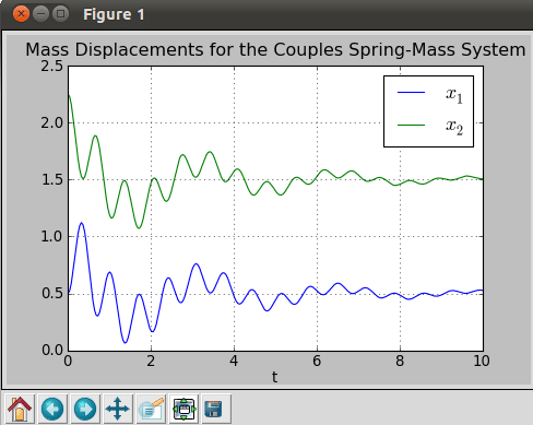
On running the script, we get the plot shown in Figure 12. It clearly shows how the mass displacements are reduced with time for damped systems.

In this article, we have covered some of the most basic operations in scientific computing. However, we can also model and simulate more complex problems with NumPy and SciPy. These tools are now actively used for research in quantum physics, cosmology, astronomy, applied mathematics, finance and various other fields. With this basic understanding of scientific programming, you’re now ready to explore deeper realms of this exciting world!