The H2O project developed by H20.ai provides users tools for data analysis, allowing them to fit thousands of potential models when trying to discover patterns in data. It is a very versatile tool since it is supported by various programming languages like R, Python and MATLAB.
Deep learning is a superset of the artificial neural network architecture and is gradually becoming an essential tool for data analysis and prediction. Leading programming languages like R, Python and MATLAB provide powerful tools and support for the implementation of data analysis using deep learning. Among such different tools, both TensorFlow and H2O have supportive packages in R and Python. Hence, both these languages are steadily becoming indispensable for deep learning and data analysis.
Deep learning with H2O
The main objective of H2O.ai is to add intelligence to business. This works on the principle of deep learning and computational artificial intelligence. H2O provides easy solutions for data analysis in the financial services, insurance and healthcare domains, and is gradually proving itself as an efficient tool for solving complex problems.
This deep learning tool follows the multi-layer feed forward neural networks of predictive models, and uses supervised learning models for regression analysis and classification tasks. To achieve process-parallelism over large volumes of data distributed over a cluster or grid of computational nodes, it uses the MapReduce algorithm. With the help of various mathematical algorithms, MapReduce divides a task into small parts and assigns them to multiple systems. H2O is scalable from small PCs to multi-core servers and even to multi-core clusters. To prevent over-fitting, different regularisation techniques are used. Commonly used approaches are L1 and L2 (Lasso and Ridge). Other than these approaches, H2O uses the dropout, HOGWILD! and model averaging methods also. For non-linear activation functions, H2O uses the Hyperbolic tangent, Rectifier Linear and Maxout functions. The performance of each function depends on the operational scenarios and there is no one best rule to base one’s selection upon. For error estimation, this model uses either one of the Mean Square Error, Absolute, Huber or Cross Entropy functions. Each of these loss functions are strongly associated with a particular data distribution function and are used accordingly.
H2O provides both manual and automatic optimisation modes for faster and a more robust convergence of network parameters to data analysis and classification problems. To reduce oscillation during the convergence of network parameters, H2O uses the Learning Rate Annealing technique to reduce the learning rate as the network model approaches its goal.
H2O performs certain essential preprocessing of data. Other than categorical encoding, it also standardises data with respect to its activation functions. This is essential, as most of the activation functions generally do not map data into the full spectrum of the real numbers scale.
H2O and R
H2O supports standalone as well as R, Python and Web based interfaces. Here I shall discuss H2O in the R language platform. It is installed from the CRAN site with the install.packages(“h2o”) command from the command line. After successful installation, the package is loaded into the current workspace by the library (h2o) function call. Since H2O is a multi-core distributed system and can be loaded in a cluster of the system, it is invoked into the present computation environment by the h2o.init() command. In this case, to initialise the package into the local machine with all its available cores, h2o.init(nthreads = -1) is used. The ‘-1’ indicates all the cores of the local host. By default, H2O uses two cores. In case H2O is installed in a server, the h2o.init() function can establish a connection between the local host and the remote server by specifying the server’s IP address and port number as follows:
h2o.init(ip=”172,16,8.90”, port=5453)
Example: To demonstrate the strength and perfection of the deep learning approach here, I have taken up a problem related to optical character recognition (OCR). In general, OCR software first divides an alphabetic document into a grid containing a single character (glyph) in each cell. Then it compares each glyph with a set of all the characters to recognise the character of the glyph. The characters are then combined back into words and the system performs spelling and grammar checks as final processing.
The objective of this example is to identify each of the black-and-white rectangular pixels displayed as one of the 26 capital letters in the English alphabet. The glyph images are based on 20 different fonts and each letter within these 20 fonts has been randomly distorted to produce a file of 20,000 unique stimuli. Each stimulus has been converted into 16 primitive numerical attributes called statistical moments and edge counts, which have then been scaled to fit into a range of integer values from 0 through 15.
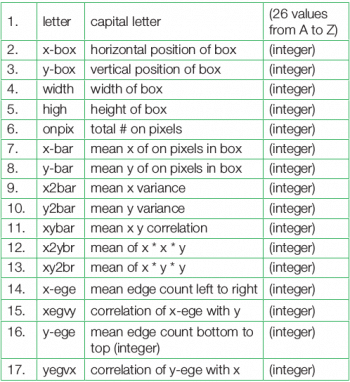
For this example, the first 16,000 items are taken for training of the neural model and then the trained model is used to predict the category for the remaining 4000 font-variations of the 26 letters of the English alphabet. The used data set is by W. Frey and D.J. Slat and is available from http://archive.ics.uci.edu/ml/datasets/Letter+Recognition. Each character is represented by a glyph and the task is to match each with one of the 26 English letters for their classification. There are 20,000 rows and 17 attributes of the character data set, as shown in Table 1.
Classification using H2O
The 16 attributes (2nd-17th rows) as stated in the above table measure different dimensional characteristics of the glyph (1st row)—the proportions of black versus white pixels, and the average horizontal and vertical position of the pixels, etc. We have to identify the glyph on the basis of these attributes, and then classify all the similar glyphs to one of the 26 characters.
To start with, first set the environment with the desired working directory and load the necessary libraries.
>path<- “I:\\DEEPNET”

>setwd(path)

>library(data.table)

>library(h2o)

>localH2o <- h2o.init(nthreads = -1)
Then download the letters.csv file from the above data archive. As per the requirements for H2O, the data set is then converted to the H2O data frame.
letterimage<- fread(“letterdata.csv”, stringsAsFactors = T)

letter.h2o <- as.h2o(letterimage)
Now it is time to set the dependent and independent variables from the letter data frame ‘letterimage’. The first column containing the English letters is the dependent variable and the rest of the columns are the independent variables.
#dependent variable (Letter)

>y.dep<- 1

#independent variables (dropping ID variables)

>x.indep<- c(2:ncol(letterimage))
To simulate the deep learning model, the H2O data frame letter.h2o is divided into training and test data sets. First, 16,000 rows are assigned to the training data set and the remaining 4000 records are considered as the test data set.
>train<- letter.h2oframe[1:16000,]

>test<- letter.h2o[16001:nrow(letter.h2oframe),]
Now we are ready to form the deep learning neural network model. The H2O function h2o.deeplearning() is used here to create a feed-forward multi-layer artificial neural network model on the training H2O data frame ‘train’.
>dlearning.model<- h2o.deeplearning

(

y = y.dep,

x = x.indep,

training_frame = train,

epoch = 50,

hidden = c(100,100),

activation = “Rectifier”,

seed = 1122

)
This function forms a neural model with two hidden layers with [100,100] synaptic nodes. The activation function of the model is set to the rectifier function. The initialisation of weightage and bias vectors has been done with random number sets with the seed value 1122. The model also sets the maximum number of iterative epochs over the model as 50. The training data set, along with the response and predictor variables (x, y), tunes the model as a universal classifier to identify and classify letters into their respective categories. The performance of the model can be studied with the help of the h2o.performance() function. To give you an idea about its performance, this function is used here over the created model itself.
>h2o.performance(dlearning.model)
This model can now be used over the test data to verify the performance of this deep neural model. The final performance study is done by comparing the outcome of the model with the actual test data. As comparison requires variables in the R data.frame format, both the predicted and the test data are converted into data frames.
>predict.dl2 <- as.data.frame(h2o.predict(dlearning.model, test))

>test.df<- as.data.frame(test)
A thorough look into both the data frames is helpful to gauge the correctness of the classification task. Often the verification of the performance is done by the confusion matrix. This is done by factorising both the data frames with the help of the table function, as shown in Table 2.
>table(test.df[,1],predict.dl2[,1])
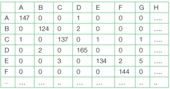
From the confusion matrix it is apparent that though there are few false positive and false negation classifications, the overall performance is quite high. A tabular matrix display is also helpful to study the performance. This can be done from the test data frame with the help of the following command sequences:
>predictions <- cbind(as.data.frame(seq(1,nrow(test.df))),

test.df[,1], predict.dl2[,1])

>names(predictions) <- c(“Sr Nos”,”Actual”,”Predicted”)

>result <- as.matrix(predictions)
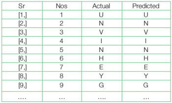 Since the number of mismatches is too low, to identify a mismatch and to study the performance it is better to use the table() function over the difference between the test and predicted values.
>performance <- test.df[,1] == predict.dl2[,1]

>table(performance)
performance
FALSE TRUE
222 3778
Performance shows that, out of 4000 test data cases, deep neural net failed to identify the correct letter only in 222 cases.
To compare the performance with other methods it is better to have a percentage evaluation of the classification task. Here is a simple way to do this.
>table(performance)*100/4000
FALSE TRUE
5.55 94.45
The result shows that the success rate of this experiment is 94.45 per cent.
In classification exercises, it is always better to have a comparative study of methods. I have done the above classification task with Support Vector Machine to explore a better alternative and to study how good this method is for this task.
Using Support Vector Machine (SVM)
SVM is also useful to classify image data. I have used the SVM model to classify the same data to compare the performance between the deep learning and SVM models. Though the performance of individual models is highly dependent on different model parameters and there is every possibility to get different results in different runs, my objective here is to gauge the performance difference between these two supervised learning schemes. Readers may explore this further by applying this experiment to other neural network models. As in the earlier case, appropriate libraries are loaded and then the training and test data are prepared.
>library(kernlab)#load SVM package

>letters_train<- letterimage [1:16000, ]

>letters_test<- letterimage [16001:20000, ]
Next, train the SVM (ksvm) with the letter column as the only response variable and the rest of the columns as predictors. As Radial Basis Function (RBF) works better for classification tasks in many cases, I have used the RBF as the SVM kernel function. Readers may use different functions, based on their preferences.
>letter_classifier_SVM<- ksvm(letter ~ ., data = letters_train, kernel = “rbfdot”)
To verify this SVM model, we can use the test data to predict the outcome of this data:
>letter_predictions<- predict(letter_classifier_SVM, letters_test)
As in the earlier case, this performance can also be verified with the confusion matrix:
>agreement<- letter_predictions == letters_test$letter

>table(agreement)
agreement
FALSE TRUE
643 3357
In percentage terms, this can be done in either of the following two ways.
1. By using the following command:
>table(agreement)*100/4000
agreement
FALSE TRUE
7.025 92.975
2. By using the prop.table() function.
From the classification results of H2O and SVM, it is apparent that both the supervised artificial neural network models methods are suitable for Optical Character Recognition classification and can be used to achieve higher performance. While H2O requires a more advanced computational platform, the requirements of SVM are less. But H2O provides a sophisticated versatile approach; so classifier models can be designed and monitored more flexibly than with the SVM approach.


