In machine learning, clustering is a technique that groups data points. Ideally, data points in a cluster should have similarities in properties or features, which differ from those not in the same cluster. This article discusses two clustering algorithms – k-means and DBSCAN.
One of the most popular techniques in data science is clustering, a machine learning (ML) technique for identifying similar groups of data in a data set. Entities within each group share comparatively more similarities with each other compared to with those from other groups. Clustering means finding clusters in an unsupervised data set. A cluster is a group of data points or objects in a data set that are similar to other objects in the group and dissimilar to data points in other clusters. Clustering is useful in several exploratory pattern-analysis, grouping, decision-making and machine-learning situations, including data mining, document retrieval, image segmentation and pattern classification. However, generally, the data is unlabelled and the process is unsupervised in clustering.
For example, we can use a clustering algorithm such as k-means to group similar customers as mentioned and assign them to a cluster, based on whether they share similar attributes, such as age, education and so on.
Some of the most popular applications of clustering include market segmentation, medical imaging, image segmentation, anomaly detection, social network analysis and recommendation engines. In banking, analysts examine clusters of normal transactions to find the patterns of fraudulent credit card usage. Also, they use clustering to identify clusters of customers – for instance, to find loyal customers versus customers who have stopped using their services.
In medicine, clustering can be used to characterise patient behaviour, based on similar characteristics, so as to identify successful medical therapies for different illnesses. In biology, clustering is used to group genes with similar expression patterns or to cluster genetic markers to identify family ties. If you look around, you can find many other applications of clustering, but generally, it can be used for one of the following purposes: exploratory data analysis, summary generation or reducing the scale, outlier detection (especially to be used for fraud detection or noise removal), finding duplicates and data sets; or as a pre-processing step for either prediction, other data mining tasks or as part of a complex system.

A brief look at different clustering algorithms and their characteristics
[emaillocker]
Partitioned based clustering is a group of clustering algorithms that produces clusters, such as k-means, k-medians or fuzzy c-means. These algorithms are quite efficient and are used for medium and large sized databases. Hierarchical clustering algorithms produce trees of clusters, such as agglomerative and divisive algorithms. These groups of algorithms are very intuitive and are generally good with small-sized data sets. Density based clustering algorithms produce arbitrary shaped clusters. They are especially good when dealing with spatial clusters or when there is noise in your data set — for example, the DBSCAN algorithm.
In this article, I will take you through the types of clustering, the different clustering algorithms and compare two of the most commonly used clustering methods.
k-means clustering
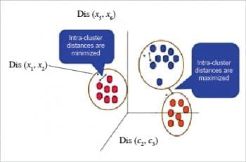
k-means is probably the most well-known clustering algorithm. It divides data into non-overlapping subsets (clusters) without any cluster internal structure. The objective of k-means is to form clusters in such a way that similar samples go into a cluster and dissimilar samples fall into different clusters. So we can say k-means tries to minimise the intra-cluster distances and maximise the inter-cluster distances.
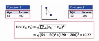
Now the question is about how to calculate the dissimilarity or distance of two cases such as two customers. We can easily use a specific type of Minkowski distance to calculate the distance of these two customers. Indeed, it is the Euclidean distance.
And what if we have more than one feature? Well, we can still use the same formula, but this time, in a two-dimensional space.
The steps involved are listed below.
- In the first step, we should determine the number of clusters. The key concept of the k-means algorithm is that it randomly picks a centre point for each cluster, which means that we must initialise ‘k’, which represents the number of clusters.
- Then, the algorithm will randomly select the centroids of each cluster.
- After the initialisation step, which defined the centroid of each cluster, we have to assign each point to the closest centre. For this purpose, we have to calculate the distance of each data point or in our case, each customer, from the centroid points, which will be assigned for each data point to the closest centroid (using Euclidean distance).
It is safe to say that this does not result in good clusters because the centroids were chosen randomly from the beginning. Indeed, the model will probably have a high error rate. Here, the error is the total distance of each point from its centroid. - So how can we turn them into better clusters with less error? We move the centroids. The main objective of k-means clustering is to minimise the distance of data points from the centroid of this cluster and maximise the distance from other cluster centroids. So in this step, we have to find the closest centroid to each data point.
- Re-compute cluster centroids: The new centroids will be calculated as the mean of the points that belong to the centroid of the previous step.
In a nutshell, the steps involved in the k-means algorithm are:
- Randomly place ‘n’ centroids, one for each cluster.
- Calculate the distance of each data point from each centroid.
- Assign each data point to its closest centroid, creating a cluster.
- Recalculate the position of centroids.
- Since k-means is an iterative algorithm, repeat Steps 2 to 4 until it results in the clusters with minimum error or the centroids no longer move.
Implementing the k-means algorithm
Initially, import the following libraries — Pandas, Numpy and Matplotlib. Next, generate some random data in a two-dimensional space. Here, a 100 data points have been generated and divided into two groups of 50 points each.
import pandas as pd
import numpy as np
import matplotlib.pyplot as plt
from sklearn.cluster import KMeans
X= -2 * np.random.rand(100,2)
X1 = 1 + 2 * np.random.rand(50,2)
X[50:100, :] = X1
plt.scatter(X[ : , 0], X[ :, 1], s = 50, c = ‘b’)
plt.show()
#In this case, we arbitrarily gave k (no of clusters) a value of two.
#Next, we need to find the centre of the clusters, centroid by using Kmean.cluster_centres

from sklearn.cluster import KMeans
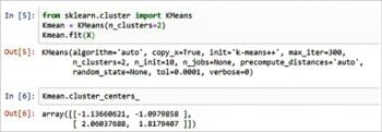
Kmean = KMeans(n_clusters=2)
Kmean.fit(X)
Kmean.cluster_centers_
#Hence we get the value of centroids, -1.13660621, -1.0979858 and 2.06037688, 1.8179407
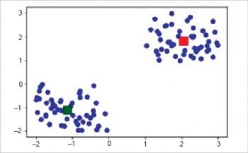
plt.scatter(X[ : , 0], X[ : , 1], s =50, c=’b’)
plt.scatter(-0.94665068, -0.97138368, s=200, c=’y’, marker=’s’)
plt.scatter(2.01559419, 2.02597093, s=200, c=’r’, marker=’s’)
plt.show()
The k-means algorithm identifies ‘k’ number of centroids and then allocates every data point to the nearest cluster, while keeping the centroids as small as possible. The ‘means’ in k-means refers to averaging of the data, i.e., finding the centroid.
The correct choice of ‘k’ is often ambiguous because it’s very dependent on the shape and scale of the distribution of points in a data set.
The elbow method is used for determining the correct number of clusters in a data set. It works by plotting the ascending values of ‘k’ versus the total error obtained when using that ‘k’. This means increasing ‘k’ will always decrease the error. So, the value of the metric as a function of ‘k’ is plotted and the elbow point is determined where the rate at which the error decreases shifts sharply. It is the right ‘k’ for clustering.
So, k-means is partition based clustering, which is relatively efficient on medium and large sized data sets. It produces sphere-like clusters because the clusters are shaped around the centroids. Its drawback is that we need to pre-specify the number of clusters, which is not going to be an easy task.
Density based clustering algorithms
Most traditional clustering techniques such as k-means, hierarchical and fuzzy clustering can be used to group data in an unsupervised way. However, when applied to tasks with arbitrary shaped clusters or to clusters within clusters, traditional techniques might not be able to achieve good results, i.e., elements in the same cluster might not share enough similarity or the performance may be poor.
In contrast, density based clustering locates regions of high density that are separated from one another by regions of low density. Density in this context is defined as the number of points within a specified radius.
DBSCAN (Density Based Spatial Clustering of Applications with Noise) is a specific and very popular type of density based clustering, which is particularly effective for tasks like class identification in a spatial context, and it can find out any arbitrary shaped cluster without getting affected by noise. Also, it is efficient for large databases.
How DBSCAN works
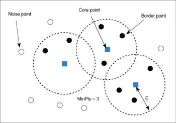
DBSCAN works on the idea that if a particular point belongs to a cluster, it should be near lots of other points in that cluster. It works based on two parameters — radius and minimum points. R or ‘eps’ determines a specified radius which, if it includes enough points within it, is called a dense area. M determines the minimum number of data points we want in a neighbourhood to define a cluster. As a general rule, the minimum M can be derived from the number of dimensions D in the data set as, M >= D+1. The minimum value of M that can be chosen is 3.
In this algorithm, we have the following three types of data points.
Core point: A point is a core point if it has more than one minimum point, M, within eps.
Border point: This is a point which has fewer than the minimum points within the radius (eps) but is in the neighbourhood of a core point.
Noise or outlier: A point that is not a core or border point.Epsilon ε or, in short, eps, indicates the radius.
The DBSCAN algorithm can be abstracted in the following steps:
- The algorithm starts with an arbitrary point which has not been visited. And if this point contains MinPts within the neighbourhood, cluster formation starts. Otherwise the point is labelled as noise.
- For each core point, if it is not already assigned to a cluster, create a new cluster.
- Identify and assign border points to their respective core points.
- Iterate through the remaining unvisited points in the data set. Points that do not belong to any cluster are noise.
 The main drawback of DBSCAN is that it doesn’t perform as well as others when the clusters are of varying density. This is because the setting of the distance threshold ε and MinPts for identifying the neighbourhood points varies from cluster to cluster, when the density varies. If the data and features are not so well understood by a domain expert, then setting up and MinPts could be tricky. Meanwhile, the DBSCAN algorithm overcomes the drawbacks of k-means, such as k-means forms spherical clusters only, is sensitive towards outliers and requires one to specify the number of clusters.
The DBSCAN clustering algorithm is demonstrated below:
import numpy as np
from sklearn.cluster import DBSCAN
from sklearn import metrics
from sklearn.datasets.samples_generator import make_blobs
from sklearn.preprocessing import StandardScaler

################################################################## #Generate sample data
centers = [[1, 1], [-1, -1], [1, -1]]
X, labels_true = make_blobs(n_samples=750, centers=centers, cluster_std=0.4,
random_state=0)

X = StandardScaler().fit_transform(X)

##############################################
# Compute DBSCAN
db = DBSCAN(eps=0.3, min_samples=10).fit(X)
core_samples_mask = np.zeros_like(db.labels_, dtype=bool)
core_samples_mask[db.core_sample_indices_] = True
labels = db.labels_

###########################################################
# Number of clusters in labels, ignoring noise if present.
n_clusters = len(set(labels)) - (1 if -1 in labels else 0)
n_noise = list(labels).count(-1)

print(‘Estimated number of clusters: ‘, n_clusters)
print(‘Estimated number of noise points: ‘, n_noise)
print(“Homogeneity: %0.3f” % metrics.homogeneity_score(labels_true, labels))
print(“Completeness: %0.3f” % metrics.completeness_score(labels_true, labels))
print(“V-measure: %0.3f” % metrics.v_measure_score(labels_true, labels))
print(“Adjusted Rand Index: %0.3f” % metrics.adjusted_rand_score(labels_true, labels))
print(“Adjusted Mutual Information : %0.3f “ %metrics.adjusted_mutual_info_score
( labels_true, labels, average_method=’arithmetic’))
print(“Silhouette Coefficient: %0.3f” % metrics.silhouette_score(X, labels))

#############################################################
# Plot result
import matplotlib.pyplot as plt

# Black removed and is used for noise instead.
unique_labels = set(labels)
colors = [plt.cm.Spectral(each)
for each in np.linspace(0, 1, len(unique_labels))]
for k, col in zip(unique_labels, colors):
if k == -1:
col = [0, 0, 0, 1]
class_member_mask = (labels == k)
xy = X[class_member_mask & core_samples_mask]
plt.plot(xy[:, 0], xy[:, 1], ‘o’, markerfacecolor=tuple(col), markeredgecolor=’k’, markersize=14)
xy = X[class_member_mask & ~core_samples_mask]
plt.plot(xy[:, 0], xy[:, 1], ‘o’, markerfacecolor=tuple(col),markeredgecolor=’k’, markersize=6)

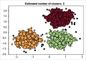
plt.title(‘Estimated number of clusters: %d’ % n_clusters)
plt.show()
The output is:
Estimated number of clusters: 3
Estimated number of noise points: 18
Homogeneity: 0.953
Completeness: 0.883
V-measure: 0.917
Adjusted Rand Index: 0.952
Adjusted Mutual Information: 0.916
Silhouette Coefficient: 0.626
To wrap up, we went through some basic concepts of the k-means and DBSCAN algorithms. A direct comparison with k-means clustering has been made to better understand the differences between these algorithms. Basically, the DBSCAN algorithm overcomes the drawbacks of the k-means algorithm.
Clustering is an unsupervised machine learning approach, but can be used to improve the accuracy of supervised machine learning algorithms. Hopefully, this will help you to get started with one of the most used clustering algorithms for unsupervised problems.
[/emaillocker]

