


In this fourth article in the ‘R, Statistics and Machine Learning’ series, we shall
explore the various ways to import data in R.
R provides various functions to load data. We shall explore reading data from CSV, JSON files and databases. We will be using R version 4.1.0 installed on Parabola GNU/Linux-libre (x86-64) for the code snippets.
$ R --version
R version 4.1.0 (2021-05-18) -- “Camp Pontanezen”
Copyright (C) 2021 The R Foundation for Statistical Computing
Platform: x86_64-pc-linux-gnu (64-bit)
R is free software and comes with ABSOLUTELY NO WARRANTY.
You are welcome to redistribute it under the terms of the
GNU General Public License versions 2 or 3.
For more information about these matters see
https://www.gnu.org/licenses/.
CSV
Consider the ‘Bank Marketing Data Set’ available from the UCI Machine Learning Repository at https://archive.ics.uci.edu/ml/datasets/Bank+Marketing. The data set is from a Portuguese banking institution and is available freely for public research use. There are four data sets available, and we will use the read.csv() function to import the data from a ‘bank.csv’ file into a data frame, as shown below:
> bank <- read.csv(file=”bank.csv”, sep=”;”)

> bank[1:3,]
  age        job marital education default balance housing loan  contact day
1  30 unemployed married   primary      no    1787      no   no cellular  19
2  33   services married secondary      no    4789     yes  yes cellular  11
3  35 management  single  tertiary      no    1350     yes   no cellular  16
  month duration campaign pdays previous poutcome  y
1   oct       79        1    -1        0  unknown no
2   may      220        1   339        4  failure no
3   apr      185        1   330        1  failure no
There are multiple options that you can pass to the ‘read.csv’ method. They are explained below:
- file: This represents the source of the file name from which the data is to be read. In our example, it is ‘bank.csv’.
- header: This is a Boolean condition which specifies if the file contains the names of the columns. In ‘bank.csv’, the header consists of:
> colnames(bank)
 [1] “age”       “job”       “marital”   “education” “default”   “balance”
 [7] “housing”   “loan”      “contact”   “day”       “month”     “duration”
[13] “campaign”  “pdays”     “previous”  “poutcome”  “y”
- sep: This is the character that separates the various fields in the file. For example, comma (“,”) for CSV files.
- quote: This specifies the type of quotes to be used if the characters are enclosed within a quotation.
- dec: Indicates the character to be used to separate decimal points. In Europe, the practice is to use comma (“,”) for the same.
- fill: Takes a Boolean value to indicate whether to insert blank values when there are rows of unequal length.
- comment.char: Represents the character to be used to ignore comment lines. The default value is hash (“#”).
You can get a count of the number of rows and columns in the data frame using the nrow() and ncol() functions respectively. For the bank data set, we have the following values:
> nrow(bank)
[1] 4521
> ncol(bank)
[1] 17
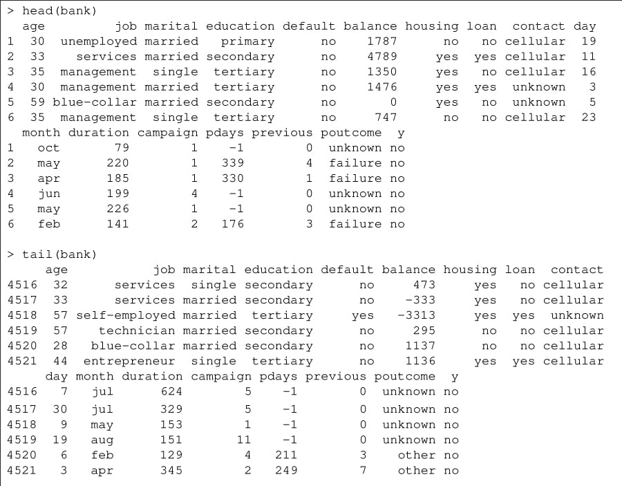
The head() and tail() functions on the data frame provide the first and last six records respectively. See Figure 1.
You can obtain the minimum and maximum values for the ‘age’ field using the following functions:
> min(bank$age)
[1] 19

> max(bank$age)
[1] 87
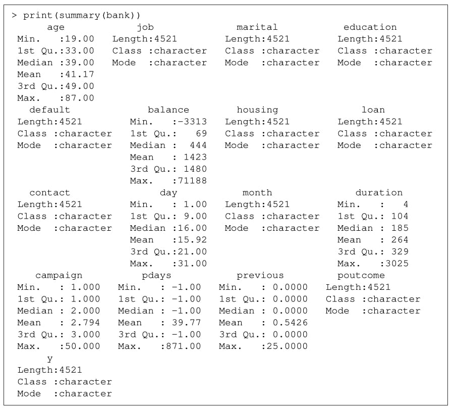
The summary() function provides information on class, mode, median, minimum, maximum for the various fields, as illustrated in Figure 2.
You can obtain a portion of the data that satisfies condition(s) using the subset() function. For example, you can find those who belong to Management, are married, have both housing and personal loans, and still maintain an annual balance of greater than 5000 Euros using the following construct:
> management <- subset(bank, job == “management” & housing == “yes” & loan == “yes” & marital == “married” & balance > 5000)

> management
     age        job marital education default balance housing loan  contact day
890   36 management married  tertiary      no    9269     yes  yes cellular  19
1601  32 management married secondary      no    6217     yes  yes cellular  18
1972  32 management married secondary      no    6217     yes  yes  unknown  21
4339  50 management married  tertiary      no   19447     yes  yes cellular  21
     month duration campaign pdays previous poutcome  y
890    nov      107        2    -1        0  unknown no
1601   nov      486        2   181        2  failure no
1972   may      486        2    -1        0  unknown no
4339   nov      166        1    -1        0  unknown no
The read.csv2() R function uses semicolon (“;”) as the default value for the separator character.
JSON
R provides support to handle JSON files. A number of libraries are available, and we will install the jsonlite library to read and process JSON files.
 > install.packages(“jsonlite”)
 Installing package into ‘/home/shakthi/R/x86_64-pc-linux-gnu-library/4.1’
 (as ‘lib’ is unspecified)
 --- Please select a CRAN mirror for use in this session ---
 trying URL ‘https://cloud.r-project.org/src/contrib/jsonlite_1.7.2.tar.gz’
 Content type ‘application/x-gzip’ length 421716 bytes (411 KB)
 ==================================================
 downloaded 411 KB

 * installing *source* package ‘jsonlite’ ...
 ** package ‘jsonlite’ successfully unpacked and MD5 sums checked
 ** using staged installation
 ** libs
 ...
 * DONE (jsonlite)
You can now load the library into the R session using:
> library(“jsonlite”)
The following JSON file is an example that provides information on colours:
[{
 “color”: “black”,
 “category”: “hue”,
 “type”: “primary”,
 “code”: {
   “rgba”: [255,255,255,1],
   “hex”: “#000”
 }
},
{
 “color”: “white”,
 “category”: “value”,
 “code”: {
   “rgba”: [0,0,0,1],
   “hex”: “#FFF”
 }
},
{
 “color”: “red”,
 “category”: “hue”,
 “type”: “primary”,
 “code”: {
   “rgba”: [255,0,0,1],
   “hex”: “#FF0”
 }
},
{
 “color”: “blue”,
 “category”: “hue”,
 “type”: “primary”,
 “code”: {
   “rgba”: [0,0,255,1],
   “hex”: “#00F”
 }
},
{
 “color”: “yellow”,
 “category”: “hue”,
 “type”: “primary”,
 “code”: {
   “rgba”: [255,255,0,1],
   “hex”: “#FF0”
 }
},
{
 “color”: “green”,
 “category”: “hue”,
 “type”: “secondary”,
 “code”: {
   “rgba”: [0,255,0,1],
   “hex”: “#0F0”
 }
}]
You can load the same in R using the fromJSON() function, as shown below:
> colors <- fromJSON(txt=”colors.json”)
> colors
   color category      type        code.rgba code.hex
1  black      hue   primary 255, 255, 255, 1     #000
2  white    value      <NA>       0, 0, 0, 1     #FFF
3    red      hue   primary     255, 0, 0, 1     #FF0
4   blue      hue   primary     0, 0, 255, 1     #00F
5 yellow      hue   primary   255, 255, 0, 1     #FF0
6  green      hue secondary     0, 255, 0, 1     #0F0
The ‘fromJSON’ function has support for a number of arguments:
- txt: This is a JSON string, URL or a file name that contains JSON.
- flatten: This is a Boolean with TRUE or FALSE that automatically flattens nested data frames.
- dataframe: This specifies how to encode data.frame objects. It should be either ‘rows’, ‘columns’ or ‘values’.
- matrix: Encoding and higher dimensional arrays should either be ‘rowmajor’ or ‘columnmajor’.
- Date: Formats that are applicable are ‘ISO8601’ or ’epoch’.
- null: Values within a list must either be ’null’ or ’list’.
- na: Values can be ‘null’ or ‘string’.
- digits: Specifies the maximum number of digits after the decimal point that should be printed.
- pretty: Indentation with whitespace for JSON output.
You can get the type of the ‘colors’ object using the typeof() function as shown below:
> typeof(colors)
[1] “list”
The number of rows, columns and column names are shown in the following output:
> colnames(colors)
[1] “color” “category” “type” “code”
> nrow(colors)
[1] 6
> ncol(colors)
[1] 4
You can obtain the values in the ‘color’ column as follows:
> colors$color
[1] “black”  “white”  “red”    “blue”   “yellow” “green”
The hex values can be obtained using nested invocation, as shown below:
> colors$code$hex
[1] “#000” “#FFF” “#FF0” “#00F” “#FF0” “#0F0”
Database
There are two major interfaces, the R Open DataBase Connectivity (RODBC) and R DataBase Interface (DBI), available in R to interact with databases. The ‘RSQLite’ package will be installed to demonstrate connectivity using the DBI interface to an SQLite database.
> install.packages(“RSQLite”)
You now need to load the installed library using the following command:
> library(“RSQLite”)
A driver object needs to be initialised with the dbDriver() function to indicate the actual driver to use when connecting to the database.
> driver <- dbDriver(“SQLite”)
You can then create the connection to the database using the dbConnect() function as shown below:
> connection <- dbConnect(drv=driver, dbname=”Chinook_Sqlite.sqlite”)
The DBI specification recommends the use of the following arguments for authentication.
- user: This is a valid user name in the database, and the default value is the current user.
- password: This is the login password to be supplied.
- host: This is the name of the machine to connect. The default value is the local connection.
- port: Refers to the port number. The default is the local connection.
- dbname: Is the name of the database on the host or the database file name.
The details about the connection can be obtained using the dbGetinfo() function, which takes in the connection object as an argument.
> dbGetInfo(connection)
$db.version
[1] “3.36.0”

$dbname
[1] “/home/guest/Chinook_Sqlite.sqlite”

$username
[1] NA

$host
[1] NA

$port
[1] NA
The class of the driver and connection objects can be displayed using the class() function.
> class(driver)
[1] “SQLiteDriver”
attr(,”package”)
[1] “RSQLite”

> class(connection)
[1] “SQLiteConnection”
attr(,”package”)
[1] “RSQLite”
A number of tables exist in the example Chinook database, as shown below:
$ sqlite3 Chinook_Sqlite.sqlite
SQLite version 3.36.0 2021-06-18 18:36:39
Enter “.help” for usage hints.

sqlite> .tables
Album          Employee       InvoiceLine    PlaylistTrack
Artist         Genre          MediaType      Track
Customer       Invoice        Playlist
You can also list the available tables from R using the dbListTables() function as follows:
> dbListTables(connection)
 [1] “Album”         “Artist”        “Customer”      “Employee”
 [5] “Genre”         “Invoice”       “InvoiceLine”   “MediaType”
 [9] “Playlist”      “PlaylistTrack” “Track”
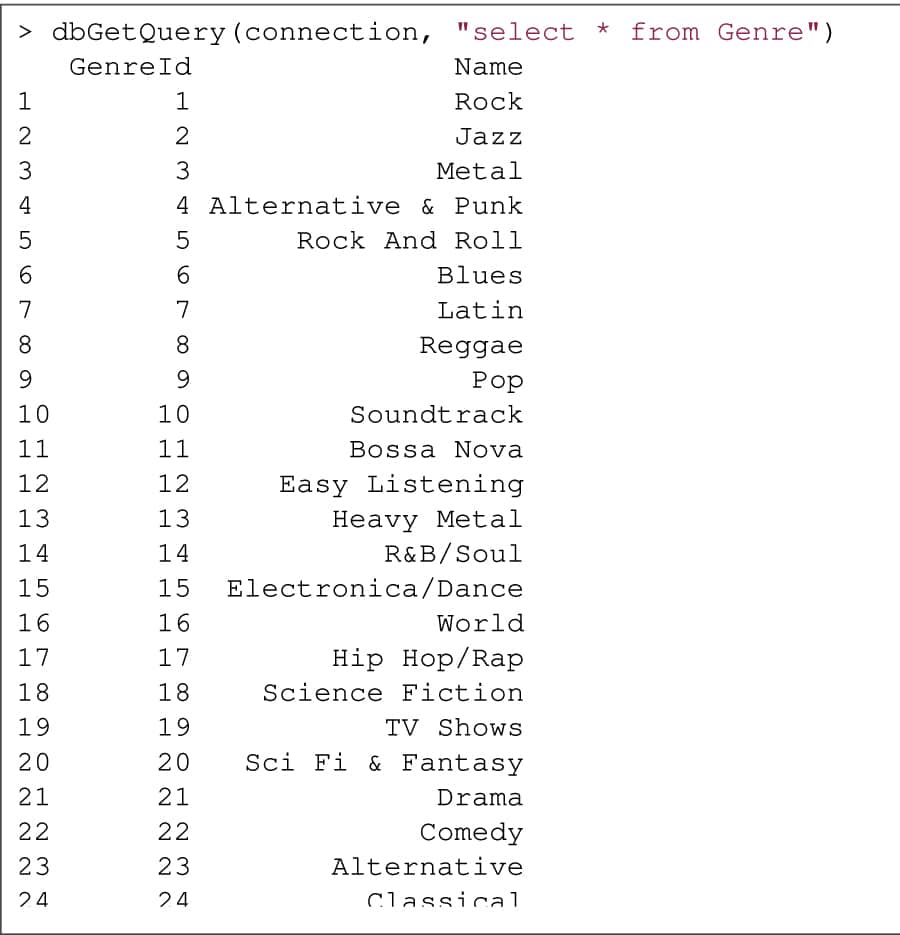
The dbGetQuery() function takes the connection object as an argument and the actual query to execute on the database, as shown in Figure 3.
Finally, you can close the database connection, unload the database driver and free memory using the dbDisconnect() and dbUnloadDriver() methods:
> dbDisconnect(connection)
> dbUnloadDriver(driver)
You are encouraged to try the above R libraries on your CSV, JSON files and databases, read the references, and the respective R library documentation for more information.


