


Python is one of the most versatile and capable computer programming languages in use today. This article dives into the world of audio waves and plays with them using Python.
Voice-controlled devices and applications are in demand today as they help to remotely access smart home devices, give navigation commands to robots and autonomous vehicles, and so on. Audio signal processing is booming, be it for industrial applications, health care, the financial sector, etc. In this article, we are going to get an insight into the use of Python tools for audio processing. We begin with an overview of this field and then move to the implementation aspects.
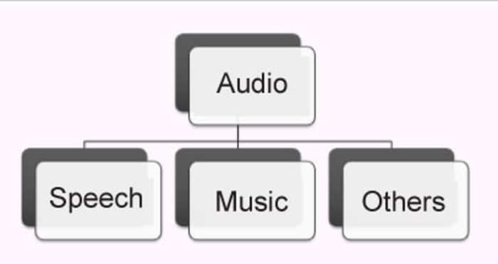
An audio signal can be categorised into: (i) speech uttered by humans (also referred to as voice), (ii) music generated by an instrument, (iii) other sounds such as a dog barking, birds chirping, surrounding noise including environmental noise, machinery sounds, etc (Figure 1). In this article, we restrict ourselves to speech and music signals; however, the processing methodology of all such files remains the same.
Speech perception in humans
Speech perception refers to the hearing ability of humans, and is mainly done through the ears. However, the structure of the human ear is complex. The outer ear is what we see. The middle ear is like a path for sound to travel towards the inner ear. The inner ear contains the most sensitive part of the human perception system, known as the cochlea. It is a snail-like structure that contains basilar membranes which act like frequency receptors. The hair cells in these membranes activate at specific frequencies, and are arranged in a logarithmic scale such that they have higher resolution at lower frequencies and lower resolution at higher frequencies. Due to this arrangement, humans find it difficult to distinguish between two different frequency tones in the higher ranges. For example, it is easy to perceive the tonal difference between two sounds having frequencies 100Hz and 200Hz, which are 100Hz apart. However, it becomes almost impossible for humans to distinguish between two sounds with frequencies 10kHz and 10.1kHz, which are also 100Hz apart. This phenomenon of human auditory nerves is imitated by Mel frequency cepstral coefficients (MFCC) features. Human ears can perceive sounds that range in frequency from 20Hz to 20kHz.
Concept of framing
An audio signal is a digital signal which comprises multiple instantaneous frequencies. Thus, it is a non-stationary signal. In order to apply signal processing algorithms, we need to divide the entire signal into short duration segments, referred to as frames. These frames are typically of 20-25ms duration with an overlap of 10ms. For each frame, a stationarity assumption is made so that the feature extraction algorithms may be executed on them. A segment larger than 30ms may not preserve the stationarity principle due to the involvement of multiple frequency components, and segment length lower than 20ms may not be adequate enough to extract features properly. Researchers experiment on frame durations ranging from 20ms to 30ms, and choose the value that optimises their solution. The framing process of an audio signal is shown in Figure 2.
![Illustration of framing process in audio signals [10]](https://www.opensourceforu.com/wp-content/uploads/2022/01/Figure-2-Illustration-of-framing-process-in-audio-signals-10.jpg)
Total # frames = Total duration of the signal (in sec) / frame size (ms)
For example, if the frame duration is 25ms and the signal is 3 seconds long, then this signal will be represented by 120 frames
Librosa
Librosa is a Python based toolkit that provides several utilities to handle audio files. It can be used to load the audio and plot the waveform of the audio file, by plotting spectrograms and varying the audio files. Let’s now see how the visualisation of a sound file is done using Librosa.
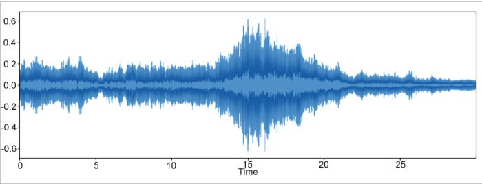
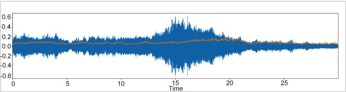
To plot the waveform of an audio file, we first need to load the audio and then pass it to the plot waveplot function. Waveplot tells us the amplitude of sound around various time intervals. In the following code, the file name can be replaced with the actual name of the wav file.
Import librosa
file=librosa.load(‘filename’)
librosa.display.waveplot(file)
Amplitude envelope
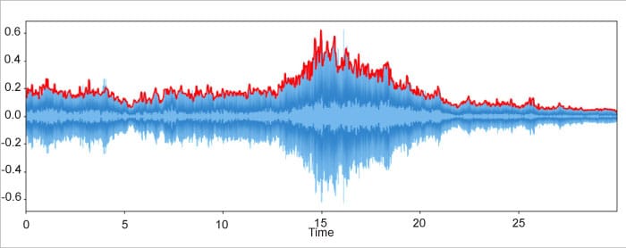
The amplitude envelope extracts the maximum amplitude within each frame and merges these together. It is important to remember that the amplitude represents the loudness of the signal. First, we split the signal into its constituent frames and find the maximum amplitude within each frame. From there, we plot the maximum amplitude in each frame along with time. The amplitude envelope can be used for onset detection or detecting the beginning of the sound. This could be external noise, someone speaking or the beginning of a musical note. The main drawback of the amplitude envelope is that it is sensitive to the outliers.
def amplitude_envelope(signal,frame_length,hop_length):
 	max_amplitude_frame=[]
  	for i in range(0,len(signal),hop_length):
    	   max_amplitude_frame.append(max(signal[i:i+frame_length]))
  return np.array(max_amplitude_frame)
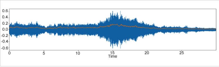
Root mean square energy (RMS)
This is somewhat similar to the amplitude envelope. As opposed to detecting the beginning of a sound, it aims at perceiving the loudness for event detection. Also, it is not sensitive to outliers like amplitude envelopes. To calculate RMS energy within a frame, we first square the amplitudes within the frame and then sum them up. We then divide this figure by the total number of samples in the frame and take the square root, which gives us the RMS energy of that specific frame.
librosa.feature,rms(signal,frame_length,hop_length)
Zero crossing rate (ZCR)
The ZCR studies the rate at which a signal’s amplitude changes within a frame. It can be used for identifying the percussion sound in music, as signals of that type of sound often have a fluctuating crossing rate. However, this feature is often used in human speech detection. To calculate the ZCR in a specific frame, we apply the sigmoid function to two continuous samples and divide their summation by 2.
librosa.feature,zero_crossing_rate(signal,frame_length, hop_length)
Fourier transform and spectrogram
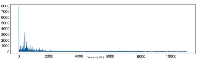
The features described above do not provide any information on the frequency of the given signal. To get that information, we apply the discrete Fourier transform on the audio signal, which provides us with the frequency and magnitude of each frequency component in the audio signal. The code for plotting the magnitude spectrum of our audio signal is given below:
def plot_magnitude_spectrum(signal, sr, title, f_ratio=1):
    X = np.fft.fft(signal)
    X_mag = np.absolute(X)
    plt.figure(figsize=(18, 5))
    f = np.linspace(0, sr, len(X_mag))
    f_bins = int(len(X_mag)*f_ratio)
    plt.plot(f[:f_bins], X_mag[:f_bins])
    plt.xlabel(‘Frequency (Hz)’)
    plt.title(title)
Spectrograms using Librosa
The frequency spectrum (Figure 7) shows the frequency domain. However, to obtain more details of the signal, we employ time-series analysis in the form of spectrograms. A spectrogram is a visual representation of the spectrum of frequencies of a signal as it varies with time. Additionally, it captures amplitude variations in the signal. Spectrograms are widely used in the fields of music, speech processing and linguistics. They can be used to identify words phonetically as well as the sounds of various calls of animals. Spectrograms can be obtained by applying the short time Fourier transform (STFT). In STFT, we apply discrete Fourier transform to each specific frame and show the results accordingly.
def plot_spectrogram(Y, sr, hop_length, y_axis=”linear”):
    plt.figure(figsize=(25, 10))
  librosa.display.specshow(Y,sr=sr,hop_length=hop_length,X_axis=”time”,   y_axis=y_axis)
    plt.colorbar(format=”%+2.f”)
| Representation | Details available | Details missing |
| Time domain waveform | Amplitude, time | Frequency |
| Frequency spectrum | Frequency, Amplitude | Time |
| Spectrogram | Amplitude, frequency, time |
Table 1: Information provided by the different representations of an audio signal
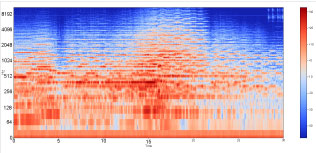
Often, signals are transformed to the frequency domain to reveal the majority of their inherent information. Time domain analysis has certain limitations, which the frequency domain can counter. Both spectrum and spectrograms are frequency domain representations of digital signals. However, in addition to time and frequency information, the latter also provide information about signal amplitude (loudness). Spectrogram based analysis is sometimes referred to as time-frequency analysis.
Voice spectrography analysis is used in crime investigations to match a suspected speaker’s voice pattern with that in criminal records. It also helps in applications such as vowel recognition based on frequency components of the signal.
| Task | Toolkits |
| Automatic speech recognition (ASR) |
Hidden Markov model (HMM) based toolkit (HTK)[1], Kaldi[2], CMU Sphinx [3] |
| Speaker diarization | DiarTK, LIUM |
| Automatic speaker recognition (ASR) and verification (ASV) | Bob, ALIZE, SIDEKIT |
| Music information retrieval (MIR) | Essentia, SMIRK |
| Common tools for audio data analysis | Audacity, Praat |
Table 2: Application-specific dedicated open source toolkits for implementing various audio processing tasks
Recent trends
Due to the pandemic, everyone prefers touch-free and hands-free interfaces for interacting with applications. Voice based devices are therefore being used for various applications. Audio spoofing detection is a recent technology, where the system checks whether the voice is generated from a genuine user or is a fake one. An interesting area of research in health care is analysing audios to determine the symptoms of any respiratory disease. In the field of music, speech-music discrimination can be done by removing or subduing the speech parts of the signal, and emphasising only the music.
Now that you have read this article, I am sure you are eager to experiment with audio signals. To begin that journey, just record your voice and play with the code given in this article. You may be amazed at what you discover along the way.


