


In this article, let’s look at the concept of linear regression with the help of an example and learn about its implementation in Python, and more.
Machine learning (ML) is a scientific study of algorithms and statistical models that computer systems use, in order to perform a specific task effectively without using explicit instructions.
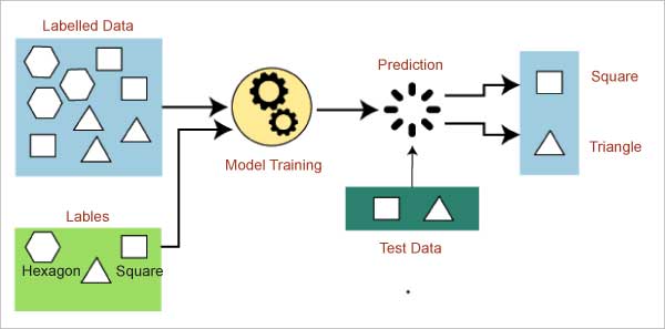
Supervised learning is a type of ML in which a machine learns from labelled data and predicts the output from those learnings. Linear regression is a popular model that comes under supervised learning. Basically, regression algorithms are used for predicting continuous variables like stock prices, weather forecasts, etc.
What is linear regression?
Regression refers to the search for relationships among variables. We can relate it to the sales of ice-cream, which are determined by the weather of the city. With an increase in humidity, ice-cream sales also rise.
In simple terms, linear regression is used for finding the relationship between two variables — the input variable (x) and the output variable (y). A single output variable can be calculated from a linear combination of multiple input variables. Input variables are also known as independent variables or predictors, while output variables are also known as dependent variables or responses.
Let us look at the simplest algorithm used for prediction.
Learning model: Ordinary least squares (OLS)
This common method can have multiple inputs. The ordinary least squares procedure seeks to minimise the sum of the squared residuals. Each time, we calculate the distance from every data point to the regression line, square it, and take the sum of all the squared errors together, ending up with considering the parameters of the least sum of all squared errors. The following example elaborates this by predicting the price of wine, given its age.
Consider the output variable (y) as the price and the input variable (x) as the age of the wine. Do remember that there could be more than one input variable. To help understand this better, we will run through an example with the values shown in Table 1.
| Age (in years) | Price (Rs) |
| 0 |
75 |
| 1.2 | 100 |
| 2.1 | 220 |
| 3.4 | 300 |
| 4.1 | 440 |
| 5.6 | 500 |
| 7 | 700 |
Table 1: The age (x) and price (y) of wine
Visualisation
The graphical representation of the data can be seen in Figure 2.
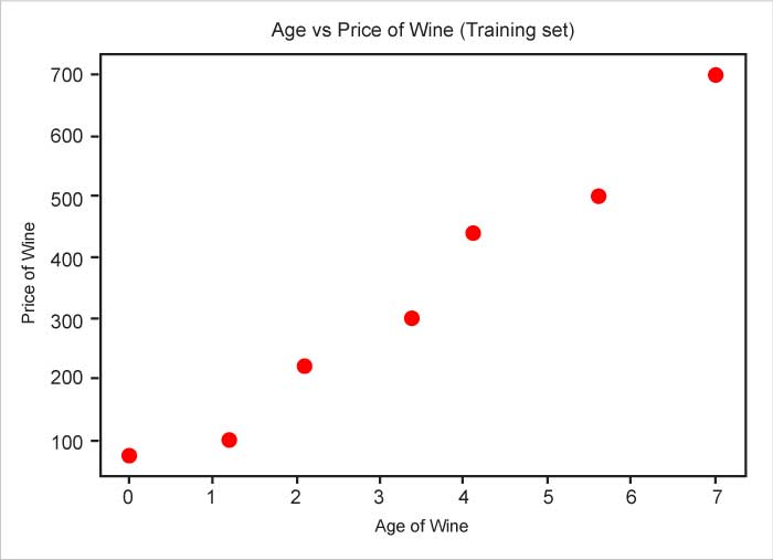
# Visualising the Training set
plt.scatter(X, y, color = ‘red’)
plt.title(‘Age vs Price of Wine (Training set)’)
plt.xlabel(‘Price of Wine’)
plt.ylabel(‘Age of Wine’)
plt.show()
We can easily see that there is a relationship between these two variables. Technically, this suggests that the variables are correlated. The correlation coefficient ‘R’ determines how strong the correlation is.
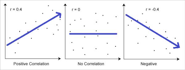
R can range from +1 to -1, but the further this figure is away from 0, the stronger is the correlation. ‘1’ indicates a strong positive relationship and ‘-1’ indicates a strong negative relationship. ‘0’, on the other hand, indicates no relationship at all.
A graphical view of a correlation of -1, 0 and +1 is shown in Figure 3.
There are several types of correlation coefficients but the most popular is Pearson’s Correlation. Its coefficient formula is seen in Figure 4.
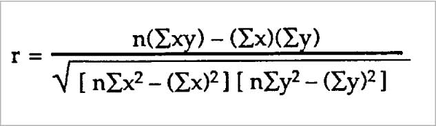
(Credits: https://www.statisticshowto.com/probability-and-statistics/correlation-coefficient-formula/#Pearson)
The two variables are divided by the product of the standard deviation of each data sample. This is the normalisation of the covariance between the two variables to give an interpretable score.
Let’s switch back to our scenario of age and price of wine to find out whether there is a correlation and, if yes, what is the value of R.
from scipy.stats import pearsonr
# calculate Pearson’s correlation
corr, _ = pearsonr(list(X.flat), y)
print(‘Pearsons correlation: %.3f’ % corr)
The output seen is:
Pearsons correlation: 0.985
The R value is 0.985, which is close to 1. Hence, the two variables are strongly positively correlated.
| Note: In simple terms, the shape of the data is important to know for selecting the model for prediction. So always draw the plot to get a sense of the data. |
Linear regression equation
Now that we have seen that our data is a good use case for linear regression, let’s have a look at the formula. The linear equation is:
y = B0 + B1*x
Here, y is the predicted variable. B0 is the intercept — the predicted value of y when x is 0. In this example, you can see that when x is 0, the value of y is 75. B1 is the regression coefficient, which refers to the change expected in y as x increases. Again going back to the example, as the number of years increases, the price of the wine also increases. Now, let’s try and find out how much it increases.
y = B0 + B1*x1 + B2*x2 + ... + BN*xN
When we have multiple input variables, as seen here, the aim of the linear regression algorithm is to find the best values for B0, B1, .. , BN.
A model ‘train, validate and test’ set
Before training our model, we need to do a train and validation split.
- Train: Set of input and output data for the model to learn.
- Validate: Set of input and output data used for evaluation of the model, to see it is not over fitted and reacting well to unseen data. It is also used for fine tuning hyper parameters, feature selection, threshold cut-off selection, and so on.
- Test: Final set of unseen data to evaluate the final model.
OLS calculation
In this method, we have to choose the values of B0 and B1 such that the total sum of squares of the difference between the calculated and observed values of y is minimised.
Before we write the source code in Python, we need to understand how the OLS works if we had to do things manually.
Step 1: Calculate the data given in Table 2 from the formulas given below, i.e., Sxx – Sum of squares of x; Syy – Sum of squares of y; and Sxy – Sum of products of x and y.
The formulas are:
- x – Mean of x
- y – Mean of y
- Sxx – Sum of squares of ( x – ˉx )
- Syy – Sum of squares of ( y – ˉy )
- Sxy – Sum of products of ( x – ˉx ) and ( y – ˉy )
-
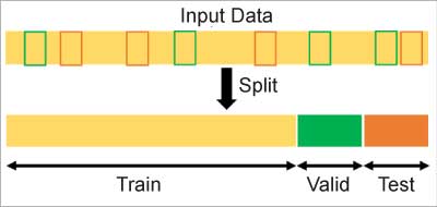
Figure 5: Randomly split the input data into a train, valid, and test set (Credits: https://towardsdatascience.com/how-to-split-data-into-three-sets-train-validation-and-test-and-why-e50d22d3e54c)
| Age of wine | Price of wine | x – ˉx | y – ˉy | ( x – ˉx ) ² | ( y – ˉy ) ² | ( x – ˉx )* ( y – ˉy ) | |
| 1 | 0 | 75 | -3.34 | -258.57 | 11.15 | 66859.18 | 864.37 |
| 2 | 1.2 | 100 | -2.14 | -233.57 | 4.57 | 54555.61 | 500.51 |
| 3 | 2.1 | 220 | -1.24 | -113.57 | 1.53 | 12898.47 | 141.15 |
| 4 | 3.4 | 300 | 0.06 | -33.57 | 0 | 1127.04 | -1.91 |
| 5 | 4.1 | 440 | 0.75 | 106.43 | 0.56 | 11327.04 | 80.58 |
| 6 | 5.6 | 500 | 2.26 | 166.43 | 5.11 | 27698.47 | 375.65 |
| 7 | 7 | 700 | 3.66 | 366.43 | 13.4 | 134269.9 | 1340.08 |
| Sum | 23.4 | 2335 | 0 (will always be zeros) | 0 (will always be zero) | 36.36 is Sxx |
308735.71 is Syy |
3300.42 is Sxy |
| Average | 3.34 is ˉx |
333.57 is ˉy |
Table 2 shows the calculation.
Step 2: Find the residual sum of squares, written as Se or RSS.
The formulas are:
- y is the observed value
- ŷ is the estimated value based on our regression equation (Note: The caret in ŷ is affectionately called a hat, so we call this parameter estimate y-hat)
- y – ŷ is called the residual and is written as e
The calculation is given in Table 3.
| Age of wine x |
Price of wine y | Predicted price of wine ŷ = B0 + B1x ŷ |
Residuals (e_ y – ŷ |
Squared residuals ( y – ŷ )^2 |
|
| 1 | 0 | 75 | B0 + B1 * 0 | 75 – (B0 + B1 * 0) | [ 75 – (B0 + B1 * 0) ] ^ 2 |
| 2 | 1.2 | 100 | B0 + B1 * 1.2 | 100 – (B0 + B1 * 1.2) | [ 100 – (B0 + B1 * 1.2) ] ^ 2 |
| 3 | 2.1 | 220 | B0 + B1 * 2.1 | B0 + B1 * 2.1 | [ 220 – (B0 + B1 * 2.1) ] ^ 2 |
| 4 | 3.4 | 300 | B0 + B1 * 3.4 | 300 – (B0 + B1 * 3.4) | [ 300 – (B0 + B1 * 3.4) ] ^ 2 |
| 5 | 4.1 | 440 | 440 – (B0 + B1 * 4.1) | 440 – (B0 + B1 * 4.1) | [ 440 – (B0 + B1 * 4.1) ] ^ 2 |
| 6 | 5.6 | 500 | B0 + B1 * 5.6 | 500 – (B0 + B1 * 5.6) | [ 500 – (B0 + B1 * 5.6) ] ^ 2 |
| 7 | 7 | 700 | B0 + B1 * 7 | 700 – (B0 + B1 * 7) | [ 700 – (B0 + B1 * 7) ] ^ 2 |
| Sum | 23.4 | 2335 | 7B0 + 16.4B1 | 2335 – (7B0 + 23.4B1) | Se |
| Average | 3.34 is ˉx |
333.57 is ˉy |
B0 + 3.34B1 is B0 + B1 ˉx |
333.57 – (B0 + 3.34B1) is ˉy – (B0 + ˉxB1) |
Se / 7 |
| Note: How the formula derivation is arrived at is out of the scope of this article. Hint: Use calculus to differentiate y = (B0 + B1x)^n with respect to x. Calculus is the mathematical study of continuous change, and differentiation cuts things into smaller pieces to find how they change. |
Step 3: Find the regression equation using the B0 and B1 formulas.
- B0 = ˉy – ˉx B1
- B1 = Sxy / Sxx
Let’s plug in the values we calculated in Step 1.
- B1 = Sxy / Sxx = 3300.43/36.36 = 90.77
- B0 = ˉy – ˉx B1 = 333.57 – (3.34 * 90.77) = 30.40
The regression equation is:
y = 30.40 + 90.77x
| Note: The values above are rounded; hence, if you run through the program there will be slight variations. Also, here we should have normalised the value of the price of wine, to see non-biased results. |
Here’s a recap of what we have seen so far.
The relationship between the residuals and the slope B1 (alias a) and intercept B0 (alias b) is always as follows.
- B1: Sum of products of x and y / sum of squares of x = Sxy / Sxx
- B0: Mean of y – mean of x * B1 = ˉy – ˉx B1
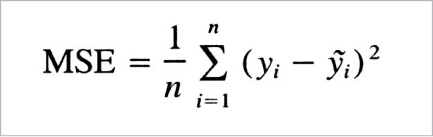
Cost function
This helps us find the best possible values of B0, B1, .., BN, from where the average is taken by all the residuals. It is also known as the mean squared error (MSE) function.
We can also use the root mean squared error (RMSE) function as a cost function.
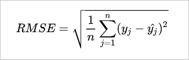
RMSE is more sensitive to outliers. But when the outliers are exponentially rare (like in a bell shaped curve), the RMSE performs very well and is generally preferred.
Correlation coefficient (R)
Now that we have the regression equation, let’s see how accurate our predictions are when we use it. As per our expectation, shown in Figure 2, the line should be closest to the dots, i.e., the predicted values should be closer to the observed values (dots).
To help understand the accuracy of the predictions, we can use the correlation coefficient R to represent the accuracy of a regression equation. This is the same function used before to check the correlation of the data to make sure the linear regression model is a suitable candidate for this data.
The formulas are:
R = sum of products y and ˉy / root of sum of squares of y and sum of squares of ˉy
Data: B1 = Sxy / Sxx = 3300.43/36.36 = 90.77
B0 = ˉy – ˉx B1 = 333.57 – (3.34 * 90.77) = 30.40
The calculation is given in Table 4.
| Age of wine x |
Price of wine y |
Predicted price of wine ŷ = B0 + B1xŷ = 30.40 + 90.77x |
Residuals (e = y – ŷ |
Squared residuals ( y – ŷ )^2 |
|
| 1 | 0 | 75 | 30.11 | 44.89 | 2014.8 |
| 2 | 1.2 | 100 | 139.05 | -39.05 | 1524.68 |
| 3 | 2.1 | 220 | 220.75 | -0.75 | 0.56 |
| 4 | 3.4 | 300 | 338.76 | -38.76 | 1502.24 |
| 5 | 4.1 | 440 | 402.3 | 37.7 | 1421.04 |
| 6 | 5.6 | 500 | 538.47 | -38.47 | 1479.97 |
| 7 | 7 | 700 | 665.56 | 33.44 | 1186.15 |
| Sum | 23.4 | 2335 | |||
| Average | 3.34 is ˉx |
333.57 is ˉy |
Se / 7 = 9129.42 |
To check how much variance is explained by our regression equation, we use R^2. This is also called the coefficient of determination.
Model training
It’s really simple to code in Python, since all the functions to be used are already written. We will be using the module named sklearn for the task.
from sklearn.linear_model import LinearRegression
lm = LinearRegression()
lm.fit(X_train, y_train)
y_pred = lm.predict(X_test)
Here, X_train is the training input; y_train is training expected output; X_test is testing input; y_test is testing actual output; and y_pred is testing predicted output.
The methods used are:
- LinearRegression(): This fits a linear model with coefficients B = (B1, …, BN) to minimise the residual sum of squares between the observed targets in the data set and the targets predicted by the linear approximation.
- fit(): This method fits the model to the input training instances.
- predict(): This performs predictions on the testing instances, based on the parameters learned during fit.
The output source code is:
y_pred
	array([ 30.11355599, 139.04715128, 220.74734774, 338.75874263,402.30333988, 538.47033399, 665.55952849])

print(“Coeffient(B1) {} and Intercept(B0) {}”.format(lm.coef_, lm.intercept_))
Coeffient(B1) [90.77799607] and Intercept(B0) 30.11355599214147
Predictions
Now that we have trained our model, let’s see how close to the truth the predictions are.
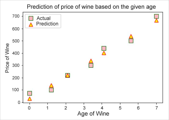
plt.title(‘Prediction of Price of Wine based on the given Age’)
plt.xlabel(“Age of wine”) #x label
plt.ylabel(“Price of wine”) #y label

plt.scatter(X_test, y_test, c =”pink”,
            marker =”s”,
            edgecolor =”green”,
            s = 100,
            label = “Actual”)
plt.scatter(X_test, y_pred, c =”yellow”,
            marker =”^”,
            edgecolor =”red”,
            s = 80,
            label = “Prediction”)
plt.legend()
Though the model performed really well, the predictions were not completely accurate. So how confident are we about our model’s prediction? To answer this question, we need to know the ‘confidence interval’.
Generally, we don’t want our model to be 100 per cent accurate, because it will be considered as an overfit and will not generalise well.
In simple terms, assume the model is a student, who is going for an English language exam. We have given this student a few questions to learn which, coincidently, are asked in the exam. The model does well, scoring full marks.
However, this will not always be the case. If the questions are different, the model will not understand them and fail, as it has memorised only these answers verbatim.
The takeaway from here is that instead of giving a few questions, giving the whole book (i.e., more data) to the model will make memorising hard, and it will start learning and finding patterns.
The assumptions we make here are:
- Input and output variables should be numeric.
- Outliers should be removed or replaced.
- Remove collinearity between input variables (x), as linear regression will over-fit your data when you have highly correlated input variables. There should be collinearity with input and output but not within input variables.
Rescale inputs, as linear regression will often make more reliable predictions if you rescale input variables using standardisation or normalisation.


