


In the first article on this series on AI (published in OSFY, June 2022), we discussed how fields like AI, machine learning, deep learning, data science, etc, are related yet distinct from each other. We also made a few difficult choices regarding the programming language, tools, etc, which will be used throughout this series. Finally, we started discussing matrices. In this article, we will discuss more about matrix theory, the heart of AI. But before we proceed any further, let us discuss the history of AI.
first of all, why is a discussion on the history of AI essential? Well, there were a few times in history when there was great enthusiasm around research on AI, but on many of those occasions the huge expectations about the potential of AI went wrong. So, we need to learn some history of AI to understand whether this time we really are going to do wonders with AI or is it yet another bubble that is about to burst.
One important question that needs to be answered is: when did our fascination for artificial intelligence start? Was it after the invention of digital computers or did it start even before? I believe the quest for an omniscient being capable of answering all questions dates back to the beginning of civilisation. The Oracle of Delphi in the ancient times was one such supposedly divine being capable of answering all the queries asked by people. The quest for creative machines outwitting human intelligence was also fascinating to us from ancient times. There were several failed attempts to make machines capable of playing chess. For example, Mechanical Turk was an infamous fake chess playing machine constructed in the late 18th century. The inventions of logarithm by John Napier, the Pascal’s calculator by Blaise Pascal, difference engine by Charles Babbage, etc, were all predecessors to the development of artificial intelligence. Further, if you go through the history of mankind, you will find countless other real and imaginary (fake) moments hoping to achieve intelligence beyond the reach of the human brain. However, irrespective of all these achievements, the search for true AI began with the invention of digital computers.
However, if that is the case, the important question is: what were some of the milestones in the history of AI up until today? As mentioned earlier, the invention of digital computers is the single most significant event in the search for artificial intelligence. Unlike electro-mechanical devices where scalability was dependent on power requirements, digital devices simply benefited technological advancement like the transition from vacuum tubes to transistors to integrated circuits to present day very large-scale integration (VLSI) technology.
Another important phase in the development of AI could be traced back to the first theoretical analysis of AI by Allan Turing. The Turing test proposed by him suggests one of the earliest methods to test artificial intelligence. The test may not be relevant today but it was one of the first attempts to define artificial intelligence. It can be summarised as follows. Behind a curtain, there is either a person named A or a machine named B. You can talk with him/it for say 30 minutes, after which you should be able to identify whether you were conversing with a person or a machine. With the powerful chatbots of today, it is easy to see that such a test will not identify true AI. But in the early 1950s this did give a theoretical framework to understand AI.
In the late 1950s, a programming language called Lisp was developed by John McCarthy. This was one of the earliest high-level programming languages. Until then, machine languages and assembly languages (notoriously difficult to use) were used for computer programming. A very powerful machine, a very powerful language to communicate with it, and computer scientists being the optimists and dreamers made the hope for artificially intelligent machines reasonable for the first time in the history of humanity. In the early 1960s, the hopes for artificially intelligent machines were at their peak. Of course, there were a lot of developments in the computing world, but were there any wonders? Sadly, no. So, the 1960s saw hope and despair about AI for the first time. However, computer science was developing at a pace that is unparalleled in any field of human endeavour.
Then came the 70s and the 80s, where algorithms played a major role. A lot of new and efficient algorithms were developed during this period. The famous textbook ‘The Art of Computer Programming’ written by Donald Knuth (I request you to read about this person, in the world of computer science he is either Gauss or Euler) had its first volume published in the late 1960s marking the beginning of the algorithmic era. A lot of general and graph algorithms were developed during these years. Further, programming based on artificial neural networks was also introduced during this time. Though McCulloch and Pitts were the pioneers in proposing artificial neural networks as far back as the 1940s, it took decades to become a mainstream technique. Today, deep learning is almost exclusively based on artificial neural networks. Such developments in the field of algorithms led to a resurgence in research in the field of artificial intelligence in the 1980s. However, this time, limitations in communication and computing powers derailed progress in this area. For a second time, AI couldn’t live up to the huge expectations it had generated. Then came the 90s, Y2K, and the present day. Once again there is a lot of enthusiasm and hope about the positive impact of AI based applications.
Based on our discussion, it is easy to see that there were at least two other occasions in the digital era when AI was promising. On both those occasions AI didn’t live up to its expectations. Is the current enthusiasm around AI a similar one? Of course, this is a very difficult question to answer. But in my personal opinion, this time AI is going to make a huge impact. But what are the factors that made me make such a prediction? First, very powerful computing devices are cheaply available nowadays. Unlike in the 1960s or 1980s, when a handful of such powerful machines were available, we now have them in the millions and billions. Second, there are large data sets available today for training AI and machine learning based applications. Imagine an AI engineer working in the field of digital image processing in the 90s. How many digital images were available for training his/her algorithms? Well, maybe a few thousands or tens of thousands. A cursory search on the Internet will tell you that the data science platform Kaggle (a subsidiary of Google) itself has more than ten thousand data sets. The large amount of data produced on the Internet every day makes training of algorithms a lot easier. Third, high speed connectivity has made it easy to collaborate with large groups. Imagine the difficulty of computer scientists collaborating with each other until the first decade of the 21st century. The present day speed of the Internet has made collaborative AI based projects like Google Colab, Kaggle, Project Jupyter, etc, a reality. Owing to these three factors, I believe this time AI is here for good and will have some excellent applications.
More about matrices
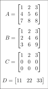
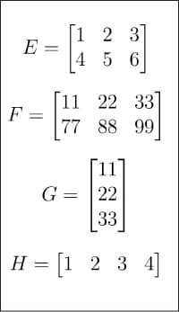
Now that we are somewhat familiar with the history of AI, it is time to revisit one of the main themes of this tutorial on AI — matrices and vectors. In the last article, we began discussing these. This time we are going to dive a little deeper into the world of matrix theory. I will begin by pointing your attention to Figures 1 and 2, which show eight matrices (A, B, C and D, and matrices E, F, G and H). Why so many matrices in a tutorial on AI and machine learning? First, as mentioned in the previous article in this series, matrices are the core of linear algebra, and linear algebra is the heart of machine learning, if not the brain. Second, each of these matrices does serve a specific purpose in the following discussion.
Let us see how matrices can be represented and how some details about them can be obtained. Figure 3 shows how matrix A is represented with NumPy. Though they are not equivalent, we use the terms matrix and array as if they are synonyms.
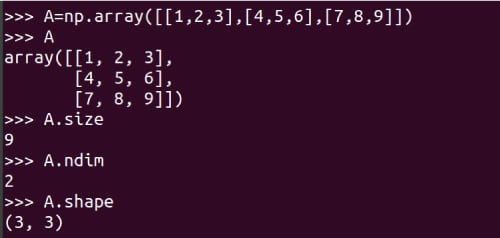
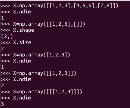
I urge you to carefully learn how a matrix is created using the function array of NumPy. There is also a function matrix offered by NumPy to create two-dimensional arrays and matrices. However, this function will be deprecated in the future and its use is no longer encouraged. We have created matrix A and Figure 3 also shows some details about it. The line of code A.size tells us about the number of elements in the array. In this case, it is 9. The line of code A.nidm tells the dimension of the array. In this case, it is easy to see that matrix A is two-dimensional. The line of code A.shape gives us the order of matrix A. The order of a matrix is the number of rows and columns of that matrix. Notice that A is a 3 x 3 matrix (3 rows and 3 columns). Though I am not explaining any further, knowing the size, dimension, and shape of an array is a little tricky with NumPy. Figure 4 shows you why the size, dimension and shape of a matrix should be identified carefully. Minor changes while defining an array could lead to changes in its size, shape, and dimension. Hence, from Figure 4, it is clear that a programmer should be extra careful while defining matrices.
Now let us perform some basic matrix operations. Figure 5 shows how two matrices A and B are added. Indeed, there are two distinct Pythonic ways to add the two matrices, either using the function add of NumPy or the operator plus (+) for matrix addition. A very important point to remember is that two matrices can be added only if they are of the same order. For example, two 4 x 3 matrices can be added whereas a 3 x 4 matrix and a 2 x 3 matrix cannot be added. However, since programming is different from mathematics, NumPy does not follow this rule in practice. Figure 5 also shows how matrices A and D are added. Remember that, in the mathematical world, this sort of matrix addition is not valid. A rule called broadcasting decides how matrices of different orders should be added. We won’t be discussing broadcasting at this point but if you are familiar with C or C++, then typecasting of variables might give you a hint as to what happens when broadcasting rules are applied in Python. So, if you want to make sure that you are performing matrix addition in the true mathematical sense, it would be safe if the following test is performed and the answer is True:
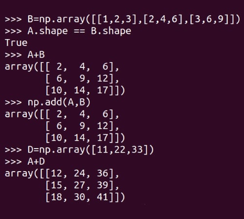
A.shape == B.shape
It can be verified that if you try to add matrices D and H, then it will give you an error.
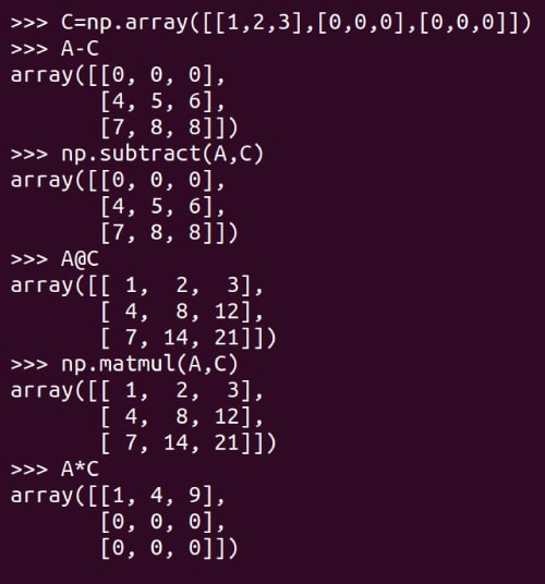
Please don’t think that matrix addition is the only operation we are going to spend time on. Of course, there are a lot more matrix operations. Matrix subtraction and multiplication are illustrated in Figure 6. Notice that subtraction and multiplication also have two distinct Pythonic ways to perform the required operations. The function subtract or the operator for matrix subtraction (-) and the function matmul or the operator for matrix multiplication (@), can be used for performing matrix subtraction and multiplication, respectively. Execution of the operator * is also shown in Figure 3. Notice that the function matmul of NumPy and the operator @ perform matrix multiplication in the mathematical sense. So, be careful with the operator * while dealing with matrices.
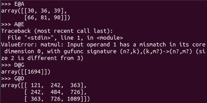
Two matrices of order (m x n) and (p x q) can be multiplied if and only if n is equal to p. Further, the product matrix will be of order (m x q). Figure 7 shows more examples of matrices being multiplied. Notice that E@A is possible whereas A@E leads to an error. Carefully go through the examples of D@G and G@D. Using the shape attribute, identify which among the eight matrices can be multiplied with each other. Though by the strict mathematical definition, a matrix is two-dimensional, we will be dealing with arrays of higher dimensions. So, just to give an example, let us see how a three-dimensional array is represented using NumPy. The following line of code creates a three-dimensional array named T.
T = np.arr ay([[[11,22],[33,44]],[[55,66],[77,88]]])
An introduction to Pandas
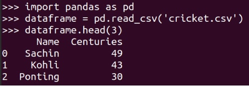
So far, we were entering matrices from the keyboard. What if we want to read a large matrix from a text file or a data set (very large for that matter) and process it? Here comes another powerful Python library to our rescue, Pandas. Let us begin by reading a small CSV (comma-separated value) file, which is a type of text file (don’t worry, soon we will read Microsoft Excel and LibreOffice/OpenOffice Calc files). Figure 8 shows how a CSV file called cricket.csv is read, and the first three lines in it are printed on the terminal. More features of Pandas will be discussed in the coming articles in this series.
Rank of a matrix
The rank of a matrix is the dimension of the vector space spanned by its rows (columns). The three italicised words, dimension, vector space and spanned, may not be familiar to you unless you remember your college level linear algebra. If you fully understand what is meant by the rank of a matrix, I am happy and no further explanation is required. However, if you are not familiar with the terms, think of it as the amount of information contained in the matrix. Again, this is a gross oversimplification and I am not proud of it. Figure 9 shows how the ranks of matrices are found out. Matrix A has rank 3 because none of its rows can be obtained from any other rows in it. Matrix B’s rank is just 1, because the second and third rows can be obtained by multiplying the first row ([1, 2, 3]) with 2 and 3, respectively. Matrix C only has one non-zero row and hence has rank 1. Similarly, the ranks of the other matrices can also be understood. Rank is very relevant in our discussion and we will revisit this topic in later articles in this series.
Now it is time for us to wind up our discussion for this month. In the next article in this series, we will add more tools to our arsenal so that they can be used for developing AI and machine learning based applications. We will also discuss terms like neural networks, supervised learning, unsupervised learning, etc, in more detail. Further, from the next article onwards, we will use JupyterLab in place of the Linux terminal.


