This article will help you understand the concept of sentiment analysis and learn how it is done. It uses different machine learning algorithms for sentiment analysis, and then compares them to decide which one is the best for the particular problem described here.
Sentiment analysis is a major area in the field of natural language processing. A sentiment is any opinion or feeling that we have about an event, a product, a situation or anything else. Sentiment analysis is the field of research in which human sentiments are automatically extracted from the text. This field started evolving in the early 90s.
This article will help you understand how machine learning (ML) can be used for sentiment analysis, and compare the different ML algorithms that can be used. It does not try to improve the performance of any of the algorithms or methods.
In today’s fast paced world, everything is online and everyone can post their views. A few negative online comments may hurt a company’s reputation and, thereby, its sales. Now that everything’s online, everyone can post their views and opinions. It becomes very important for companies to go through these to understand what their customers really want. But since there is so much data, it cannot be gone through manually. This is where sentiment analysis comes in.
Let us now start developing a model to do a basic sentiment analysis.
Let’s start!
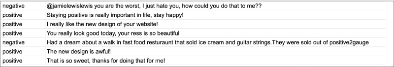
The first step is to select a data set. You can choose from any publicly available reviews or comments such as tweets or movie reviews. The two columns that should definitely be there in the data set are the label and the actual piece of text.
Figure 1 shows a small sample of how the data looks.
Now we need to import the required libraries:
import pandas as pd
import numpy as np
from nltk.stem.porter import PorterStemmer
import re
import string
As you can see in the above code, we have imported NumPy and Pandas for processing the data. We will look at the other imported libraries when we use them.
Now that the data set is ready and the libraries are imported, we need to bring the former into our project. The Pandas library is used for this purpose. We bring the data set into the Pandas data frame using the following line of code:
sentiment_dataframe = pd.read_csv(“/content/drive/MyDrive/Data/sentiments - sentiments.tsv”,sep = ‘\t’)
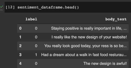
Now that we have the data set in our project, let us manipulate it so that our algorithm can understand the features better. We begin by giving names to our columns in the data set. This is done by using the line of code given below:
sentiment_dataframe.columns = [“label”,”body_text”]
We then assign numerical labels to the classes — negative is replaced with 1 and positive is replaced with 0. Figure 2 shows how the data frame looks at this stage.
The next step is the preprocessing of the data. This is a very important step as it helps us to convert string/text data into numerical data (machine learning algorithms can understand/process numerical data and not text). Also, the redundant and useless data needs to be removed as it may taint our training model. We remove the noisy data, missing values and other non-consistent data in this step.
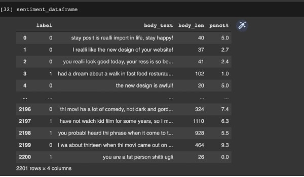
We will add the features text length and punctuation count in the data frame specifically for this application. We will also do the stemming, i.e., we will convert all similar words (like ‘give’, ‘giving’, etc) into a single form. Once this is done, we divide the data set into two — X and Y — where X is the features and Y is the prediction class.
This is done using the following piece of code. Figure 3 shows the data frame after these steps are taken.
def count_punct(text):
   count = sum([1 for char in text if char in string.punctuation])
   return round(count/(len(text) - text.count(“ “)),3)*100

 tokenized_tweet = sentiment_dataframe[‘body_text’].apply(lambda x: x.split())
stemmer = PorterStemmer()
tokenized_tweet = tokenized_tweet.apply(lambda x: [stemmer.stem(i) for i in x])
for i in range(len(tokenized_tweet)):
   tokenized_tweet[i] = ‘ ‘.join(tokenized_tweet[i])
sentiment_dataframe[‘body_text’] = tokenized_tweet
sentiment_dataframe[‘body_len’] = sentiment_dataframe[‘body_text’].apply(lambda x:len(x) - x.count(“ “))
sentiment_dataframe[‘punct%’] = sentiment_dataframe[‘body_text’].apply(lambda x:count_punct(x))
X = sentiment_dataframe[‘body_text’]
y = sentiment_dataframe[‘label’]
We now need to convert the string into numerical data. We use a count vectorizer for this purpose; that is, we get the counts of each word and convert it into a vector.
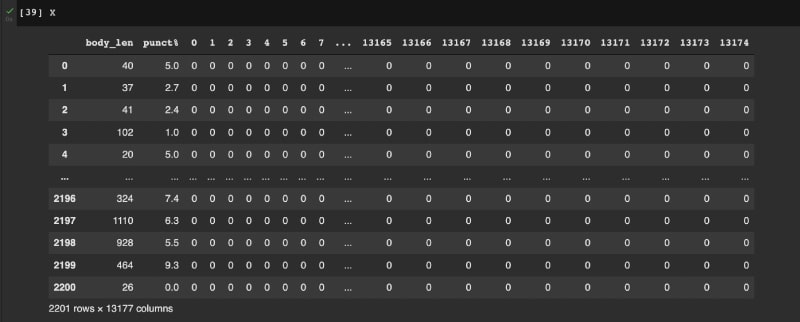
After this, features such as length of text and punctuation count in the dataframe, i.e., X, are calculated. A sample of X is shown in Figure 4.
Now the data is ready for training. The next step is to determine which algorithms we are going to use for training our model. As has been mentioned before, we are going to try several algorithms and determine the best one for sentiment analysis. Since we are basically trying to do binary classification, the following algorithms can be used:
- K-nearest neighbors (KNN)
- Logistic regression
- Support vector machines (SVMs)
- Stochastic gradient descent
- Naive Bayes
- Decision tree
- Random Forest
We first need to split our data set into testing and training data. This is done by using the sklearn library using the following code:
from sklearn.model_selection import train_test_split
X_train, X_test, y_train, y_test = train_test_split(X,y, test_size = 0.20, random_state = 99)
We will use 20 per cent of the data for testing and 80 per cent for the training part. We will separate the data because we want to test on a new set of data whether our model is working properly or not.
Now let us start with the first model. We will try the KNN algorithm first, and use the sklearn library for this. We will first train the model and then assess its performance (all of this can be done using the sklearn library in Python itself). The following piece of code does this, and we get an accuracy of around 50 per cent.
from sklearn.neighbors import KNeighborsClassifier
model = KNeighborsClassifier (n_neighbors=3)
model.fit(X_train, y_train)
model.score (X_test,y_test)

0.5056689342403629
The code is similar in the logistic regression model — we first import the function from the library, fit the model, and then test it. The following piece of code uses the logistic regression algorithm. The output shows we got an accuracy of around 66 per cent.
from sklearn.linear_model import LogisticRegression
model = LogisticRegression()
model.fit (X_train,y_train)
model.score (X_test,y_test)

0.6621315192743764
The following piece of code uses SVM. The output shows we got an accuracy of around 67 per cent.
from sklearn import svm
model = svm.SVC(kernel=’linear’)
model.fit(X_train, y_train)
model.score(X_test,y_test)

0.6780045351473923
The following piece of code uses the Random Forest algorithm, and we get an accuracy of around 69 per cent.
from sklearn.ensemble import RandomForestClassifier
model = RandomForestClassifier()
model.fit(X_train, y_train)
model.score(X_test,y_test)

0.6938775510204082
Next we use the Decision tree algorithm, which gives an accuracy of around 61 per cent.
from sklearn.tree import DecisionTreeClassifier
model = DecisionTreeClassifier()
model = model.fit(X_train,y_train)
model.score(X_test,y_test)

0.6190476190476191
The following piece of code uses the stochastic gradient descent algorithm. The output shows that we got an accuracy of around 49 per cent.
from sklearn.linear_model import SGDClassifier
model = SGDClassifier()
model = model.fit(X_train,y_train)
model.score(X_test,y_test)

0.49206349206349204
The following piece of code uses Naive Bayes. We get an accuracy of around 60 per cent.
from sklearn.naive_bayes import GaussianNB
model = GaussianNB()
model.fit(X_train, y_train)
model.score(X_test,y_test)

0.6009070294784581
Now that we have checked out all the algorithms, let us graph their accuracy performance. The graph is shown in Figure 5.
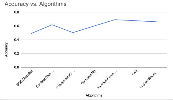
As you can see, the random forest algorithm gave the best accuracy for this problem and we can conclude that it is the best fit for sentiment analysis amongst ML algorithms. We can improve the accuracy much more by getting better features, trying out other vectorising techniques, and using a better data set or newer classification algorithms.
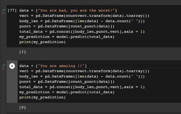
Now that random forest is seen as the best algorithm for this problem, I am going to show you a sample prediction. In Figure 6, you can see that the right predictions are being made! Do try this out to improve upon this project!