


In the previous article in this series on AI and machine learning, we explored natural language processing (NLP) using the packages PyTorch and NLTK. We also discussed PySpark and how it can be used in Big Data analytics. The main objective of this tenth article in the series on AI is to concentrate on computer vision.
By now, we have become acquainted with various types of neural networks, including FNN, CNN, RNN, LSTM, etc, among others. However, to develop AI-based applications effectively, it is essential to gain knowledge about the different types of neural network architectures. It is also important to note that the terms ‘neural network models’ and ‘neural network architectures’ are often used interchangeably, but there is a subtle difference between them. A neural network architecture is concerned with the overall design of the network, which includes the number of layers, the types of layers (fully connected, convolutional, recurrent, etc), the activation functions, and the connectivity pattern between the layers. For instance, a neural network architecture may consist of a fully connected feedforward neural network with ten hidden layers and an ReLu activation function. Many neural network models can instantiate this architecture, each with its own set of parameter values learned from the training data for a specific task.
The development of deep learning and neural network architectures is closely linked. The use of the term ‘deep learning’ in its current meaning started in the 2000s, along with the rise of deep neural network architectures. Let us now discuss some of the popular neural network architectures that have played a significant role in the history of deep learning. One of the most well-known neural network architectures is AlexNet, which gained widespread attention in 2012 when it won the ImageNet Large Scale Visual Recognition Challenge (ILSVRC 2012). This annual competition, organised by the ImageNet project, evaluates and advances the state-of-the-art in image classification and object detection tasks. AlexNet surpassed traditional computer vision algorithms by a significant margin. It is a deep neural network architecture composed of several layers, including convolutional layers, pooling layers, and densely connected layers.
VGG (Visual Geometry Group), also known as VGGNet, is a deep convolutional neural network that achieved second place in the ILSVRC 2014 contest. This architecture has been widely used as a baseline model for many computer vision tasks. In 2015, Microsoft’s Residual Neural Network (ResNet) outperformed AlexNet and won the ILSVRC 2015 contest. Other well-known neural network architectures include GoogLeNet, YOLO, and so on.
Introduction to computer vision
The survival of our species was dependent on vision, which is considered the most critical sense. If you believe in evolution, modern human beings evolved at least 300,000 years ago. Therefore, human vision was perfected over hundreds of thousands of years. But for how long has the survival of our species depended on logical reasoning? Maybe a few centuries at most — my bet is that logical reasoning became critical after the industrial revolution when skills were required for operating complex machines.
Now, why am I deviating from our discussion? Well, to state an important observation in AI and robotics called Moravec’s paradox. It states that machines are good at tasks where humans are bad, and vice versa. Chess and Go (a strategic game popular in China and other parts of East Asia) are two games that require a lot of reasoning in order to be mastered. Computer software powered by AI is today capable of beating even the best chess and Go players in the world. However, tasks like vision, motor skills, etc, which are easy for human beings, are difficult for machines to mimic.
Now, let us briefly talk about colour models, which are one of the fundamental concepts needed for computer vision and image processing. An RGB colour model uses the three primary colours of red, green, and blue to create all the other colours. We can all recall mixing primary colours of light during our school years to generate a range of colours. While the RGB model is relatively straightforward, it does not align well with human perception of colour. The HSV colour model is a better representation of how the human eye perceives colour.
In the HSV colour model, colours are defined by their hue, saturation, and value. Hue represents the dominant colour and is measured in degrees on a colour wheel, ranging from 0° to 360°. Saturation refers to the intensity of a colour and is measured as a percentage, with 0% saturation representing a shade of gray and 100% saturation representing the most intense colour possible. Value refers to the brightness of a colour and is also measured as a percentage, with 0% value representing black and 100% value representing white. To describe a colour in the HSV model, we combine the three values (hue, saturation, and value) to determine the overall appearance of the colour. For example, a bright, pure red would have a hue of 0°, a saturation of 100%, and a value of 100%. The HSV model is frequently used in digital imaging software and graphic design programs because it provides a flexible and intuitive way to manipulate and create colours. While we will not delve into the other colour models beyond RGB and HSV, it is important to understand that a thorough grasp of colour models is essential for working in computer vision. Other models like CMYK, HSL, and YUV also exist and may be useful in many situations.
Now, consider the Python script called rgb_to_hsv.py, which generates a random image similar to the one we generated in the third article in this series. But in addition to generating such an image, this Python script also converts the image to the HSV colour model (line numbers are included for ease of explanation).
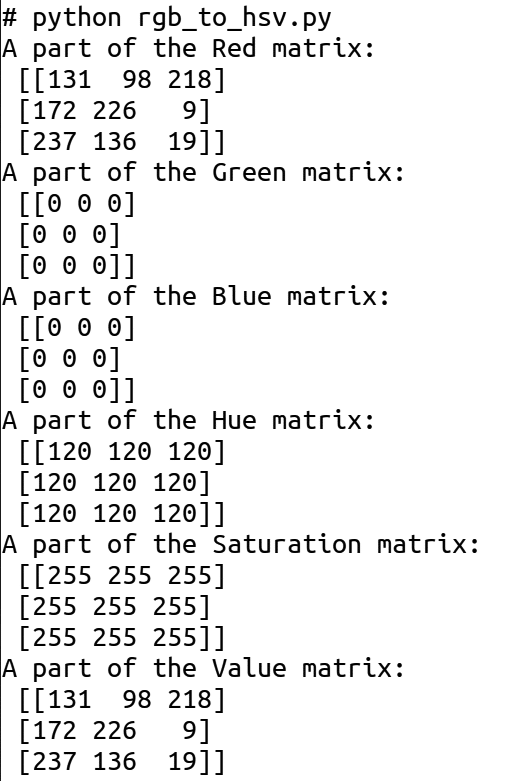
1. import numpy as np
2. import cv2
3. r_mat = np.random.randint(0, 256, size=(512, 512),dtype=np.uint8)
4. g_mat = np.zeros((512, 512),dtype=np.uint8)
5. b_mat = np.zeros((512, 512),dtype=np.uint8)
6. image = cv2.merge([r_mat, g_mat, b_mat])
7. print(“A part of the Red matrix:\n”, r_mat[:3, :3])
8. print(“A part of the Green matrix:\n”, g_mat[:3, :3])
9. print(“A part of the Blue matrix:\n”, b_mat[:3, :3])
10. hsv_image = cv2.cvtColor(image, cv2.COLOR_BGR2HSV)
11. print(“A part of the Hue matrix:\n”, hsv_image[:3, :3, 0])
12. print(“A part of the Saturation matrix:\n”, hsv_image[:3, :3, 1])
13. print(“A part of the Value matrix:\n”, hsv_image[:3, :3, 2])
Now, let us try to understand the Python script above. Lines 1 and 2 import NumPy and OpenCV. Line 3 generates a random matrix of order 256×256. Lines 4 and 5 generate two zero matrices of order 256×256. Line 6 generates an image in the RGB colour model from these three matrices. Lines 7 to 9 print a 3×3 submatrix of the red, green, and blue matrices, respectively. Line 10 converts the image from the RGB colour model to the HSV colour model. Lines 11 to 13 print a 3×3 submatrix of the hue, saturation, and value matrices, respectively. Figure 1 shows the output of this Python script. I urge you to carefully examine the matrices in the RGB and HSV colour models (shown in Figure 1) to gain further insights about these two colour models.
To further illustrate the effect of colour models, consider the Python script hsv_image.py shown below, which reads an image stored in the RGB colour model, converts it into the HSV colour model, and finally prints both the images (line numbers are included for ease of explanation).
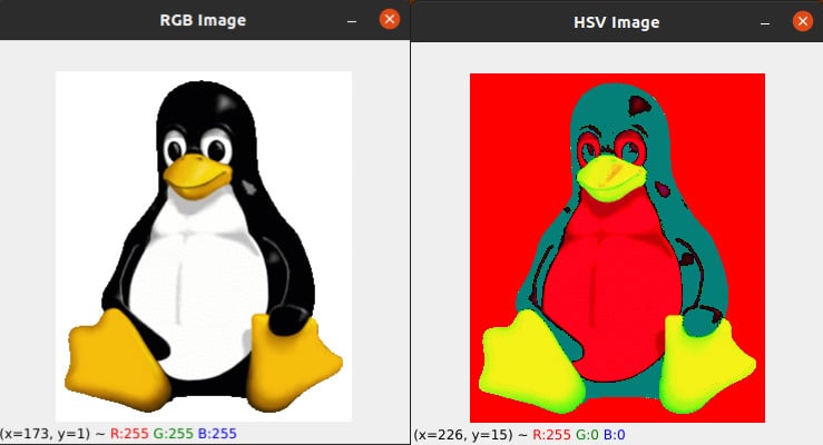
1. import numpy as np
2. import cv2
3. image = cv2.imread(“tux.png”)
4. hsv_image = cv2.cvtColor(image, cv2.COLOR_BGR2HSV)
5. cv2.imshow(“RGB Image”, image)
6. cv2.imshow(“HSV Image”, hsv_image)
7. cv2.waitKey(0)
8. cv2.destroyAllWindows( )
Now, let us try to understand the Python script above. Lines 1 and 2 import NumPy and OpenCV. Line 3 reads a file called tux.png containing the image of our familiar penguin Tux (courtesy: Wikipedia) stored using the RGB colour model, while line 4 converts this image to the HSV colour model. Lines 5 to 8 print the images in the RGB and HSV colour models. Figure 2 shows the two images generated. Let us now turn our attention to OpenCV.
Rediscovering OpenCV: A fresh introduction
In the third article in this series, we had our initial encounter with OpenCV. As a result, we are aware that OpenCV is a free and open source library that is primarily used for real-time computer vision. Starting from version 4.5.0 onwards, OpenCV is licensed under the Apache License version 2.0, while earlier versions were licensed under the BSD licence. OpenCV is a cross-platform library developed primarily using C and C++, and it includes a Python binding that allows Python developers to access the OpenCV library. OpenCV is undoubtedly one of the most widely used libraries for computer vision, if not the most widely used. We have already learned how to install and import OpenCV. Let us now examine some practical situations in which OpenCV is used in computer vision
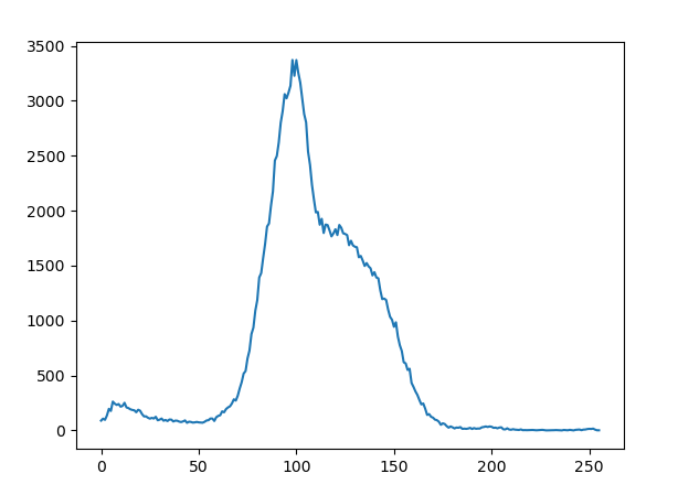
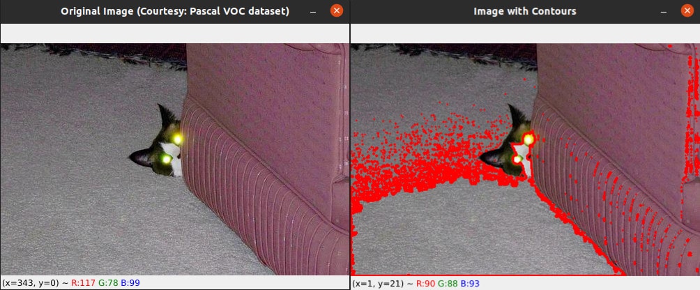
First, let us discuss image contours and image histograms. In computer vision and image processing, image contours are a set of continuous lines that form the boundary of an object or region in an image. A contour can be represented as a curve joining all the continuous points along the boundary having the same colour or intensity. Image contours can be used for object detection, recognition, and tracking. On the other hand, an image histogram is a graphical representation of the distribution of pixel intensities in an image. It represents the number of pixels in an image at different intensity levels. The horizontal axis of the histogram represents the intensity levels ranging from 0 to 255, while the vertical axis represents the number of pixels having that intensity. Image histograms can be used to analyse the brightness and contrast of an image. Consider the Python script called contour.py, shown below (line numbers are included for ease of explanation), that generates the image contours and image histogram of an image file called cat.jpg (courtesy: Pascal VOC data set).
1. import cv2
2. import matplotlib.pyplot as plt
3. image = cv2.imread(“cat.jpg”)
4. img_gray = cv2.cvtColor(image, cv2.COLOR_BGR2GRAY)
5. ret, b_img = cv2.threshold(img_gray, 127, 255, cv2.THRESH_BINARY)
6. hist = cv2.calcHist([img_gray], [0], None, [256], [0, 256])
7. cont, _ = cv2.findContours(b_img, cv2.RETR_EXTERNAL, cv2.CHAIN_APPROX_SIMPLE)
8. plt.plot(hist)
9. plt.show( )
10. cv2.imshow(“Original Image (Courtesy: Pascal VOC dataset)”, image)
11. cv2.drawContours(image, cont, -1, (0, 0, 255), 2)
12. cv2.imshow(“Image with Contours”, image)
13. cv2.waitKey(0)
14. cv2.destroyAllWindows( )
Now, let us go through the code line by line. Lines 1 and 2 import OpenCV and Matplotlib. Line 3 reads the image named cat.jpg and stores it in a variable named image. Line 4 converts the image to grayscale and stores it in a variable named img_gray. Line 5 applies a threshold to the grayscale image to convert it to a binary image with a threshold value of 127 and a maximum pixel value of 255. A binary image is an image that consists of pixels that can have one of exactly two colours, black or white. Line 6 calculates the histogram of the grayscale image using the calcHist( ) function of OpenCV. The histogram is stored in a variable called hist. The function calcHist( ) takes the following parameters: a list generated from the grayscale image to be processed ([img_gray]), the channel for which the histogram is calculated ([0]), a mask image (if None, the whole image is used), the number of bins in the histogram ([256]), and the range of pixel values ([0, 256]). Line 7 finds the contours in the binary image using the findContours( ) function of OpenCV. The contours are stored in the variable cont. The function findContours( ) takes the following parameters: the binary image (b_img), the retrieval mode (cv2.RETR_EXTERNAL denotes that only the external contours are to be retrieved), and the contour approximation method (cv2.CHAIN_APPROX_SIMPLE denotes that the contours are to be approximated by using only the endpoints of the contour segments). Lines 8 and 9 plot the histogram and display it. Line 10 displays the original image. Line 11 draws the contours on the original image in red colour using the drawContours( ) function of OpenCV. This function takes the following parameters: the original image (image), the list of contours to be drawn (contours), the index of the contour to be drawn (if the value given is -1, all the contours are drawn), the colour of the contours (here (0, 0, 255) denoting red), and the thickness of the contours (2). Lines 12 to 14 show the image with contours marked in red colour. Figure 3 shows the image histogram generated, and Figure 4 shows the original image and the modified image with contours marked in red colour.
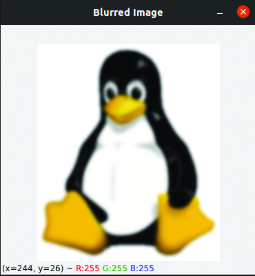
Now, let us discuss image convolution. Image convolution is a mathematical operation performed on an image to modify or enhance its features by applying a convolution kernel (a small matrix) to each pixel of the image. In a nutshell, the new value of a central pixel is obtained by operating the convolutional kernel matrix on the values of all its neighbouring pixels. A very useful example of image convolution is Gaussian blurring of images. Gaussian blurring is a popular image processing technique used to reduce image noise and sharpness by applying a Gaussian filter to the image. The Gaussian filter is a convolution matrix whose values are calculated based on the Gaussian function. Now, consider the Python script named blur.py shown below, which applies Gaussian blur to the image tux.png (line numbers are included for ease of explanation).
1. import cv2
2. image = cv2.imread(“tux.png”)
3. blur_img = cv2.GaussianBlur(image, (15, 15), 0)
4. cv2.imshow(‘Blurred Image’, blur_img)
5. cv2.waitKey(0)
6. cv2.destroyAllWindows( )
Now, let us go through the code line by line. Line 1 imports OpenCV. Line 2 reads the image tux.png. Line 3 applies Gaussian blurring on the original image using the OpenCV function GaussianBlur( ). The resulting blurred image is stored in the variable blur_img. The parameters for the function GaussianBlur( ) are as follows: the original image to be blurred (image), the size of the kernel to be used for the blurring operation (in this case, a 15×15 kernel is used), and the standard deviation of the Gaussian function used for blurring (0 indicates to OpenCV that the value should be automatically calculated based on the kernel size). Increasing the kernel size will increase the amount of blur in the resulting image. For example, you can change the second parameter of the function GaussianBlur( ) to (25, 25) to increase the blur. Adjusting the standard deviation (the third parameter of the function GaussianBlur( )) will also affect the intensity of the blur.
OpenCV provides several other blurring functions besides Gaussian blur. Some of them are box blur, median blur, etc. Replace Line 3 with the line of code ‘blur_img = cv2.blur(image, (15, 15))’ and execute the Python script to see the effect of box blur. Replace Line 3 with the line of code ‘blur_img = cv2.medianBlur(image, 15)’ and execute the Python script to see the effect of median blur. Lines 4 to 6 of the Python script blur.py display the Gaussian blurred image generated. Figure 5 shows this blurred image generated by the Gaussian filter. The image on the left of Figure 2 is the original image named tux.png, without any blurring.
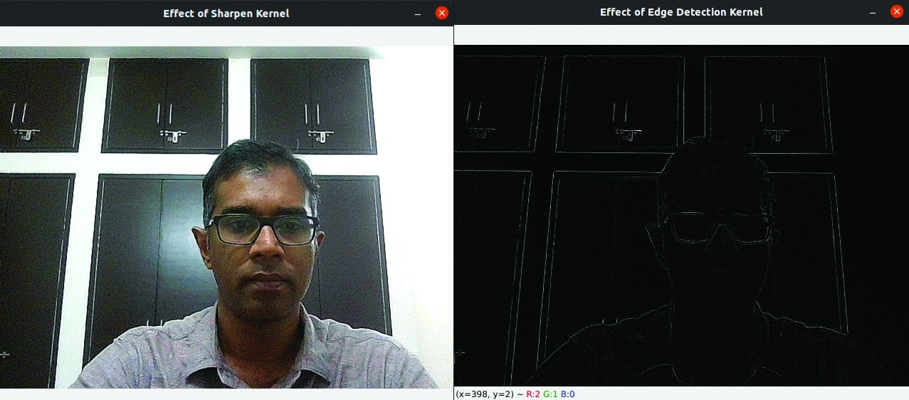
The following program further illustrates the role and importance of kernels in image processing. A kernel, also known as a convolution matrix or mask, is a small matrix used to perform tasks such as blurring, sharpening, edge detection, etc, on an image. The Python script called video.py, which reads video using your laptop camera for further processing, is shown below (line numbers are included for ease of explanation).
1. import cv2
2. import numpy as np
3. capture = cv2.VideoCapture(0)
4. while True:
5. ret, image = capture.read( )
6. cv2.imshow(“Video”, image)
7. key = cv2.waitKey(10)
8. if key == 27:
9. cv2.imwrite(“video.jpg”,image)
10. break
11. image = cv2.imread(“video.jpg”)
12. kernel1 = np.array([[0,-1,0], [-1,5,-1], [0,-1,0]])
13. kernel2 = np.array([[0,-1,0], [-1,4,-1], [0,-1,0]])
14. img1 = cv2.filter2D(image, -1, kernel1)
15. img2 = cv2.filter2D(image, -1, kernel2)
16. cv2.imshow(‘Effect of Sharpen Kernel’, img1)
17. cv2.imshow(‘Effect of Edge Detection Kernel’, img2)
18. cv2.waitKey(0)
19. cv2.destroyAllWindows( )
Now, let us go through this Python script, which captures frames using your laptop camera for further processing, line by line. Lines 1 and 2 import OpenCV and NumPy. Line 3 initialises the camera capture object to read from the default camera. Line 4 starts an infinite loop to continuously read frames from the camera. Line 5 reads a frame from the camera. Line 6 displays this image in a window named Video. Line 7 waits for 10 milliseconds for a key to be pressed and captures the key, if pressed. Lines 4 to 7 create the impression of a video composed of individual frames that have been captured. Line 8 checks if the pressed key is the escape key (ASCII code 27). If it is, Line 9 saves the current frame as a JPEG image named video.jpg, and Line 10 breaks out of the infinite loop. Line 11 reads the image saved earlier as video.jpg and stores it in a variable called image. Line 12 defines one of the most popular 3×3 sharpen kernels called the Laplacian kernel. Line 13 defines a 3×3 kernel for edge detection. Lines 14 and 15 apply the two kernels on the image using the function filter2D( ) of OpenCV and store the results in two separate variables, img1 and img2, respectively. The second parameter of the function filter2D( ) defines the desired depth of the output image. The value -1 sets the depth of the output image to be the same as the input image. Lines 16 to 19 display the two filtered images. (left: sharpen kernel and right edge detection kernel)
Figure 6 shows the two images generated by the two kernels. Take a moment to grasp the fact that the two images are drastically different from each other, even though the two 3×3 kernel matrices differ only by a single element. The importance of kernels in image processing is evident from this example, and your ability to work effectively with kernels will have a direct impact on the quality of the computer vision applications you can create.
It should be noted that our discussion regarding OpenCV is restricted to a handful of practical and basic computer vision applications. Hence, to fully comprehend the power and usefulness of OpenCV in image processing, it is highly recommended that you explore it extensively. Next, we will proceed to explore another powerful Python image processing library called scikit-image.
Introduction to scikit-image
Scikit-image is a free and open source Python library for image processing. It is licensed under the BSD licence. Scikit-image provides a wide range of image processing tools and functions for image segmentation, feature detection, image restoration, etc. But why should someone use scikit-image when OpenCV is already available? Certainly, OpenCV has been extensively optimised for performing image processing tasks in real-time. However, scikit-image has been purpose-built to cater to the needs of image processing and analysis, and is renowned for its simplicity, ease of use, and flexibility.
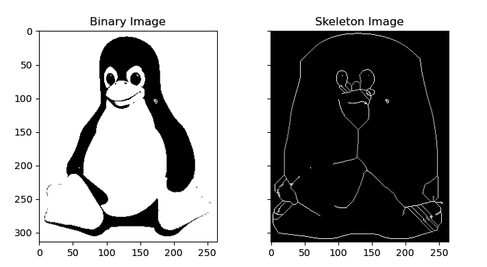
Let us now take a look at an example using scikit-image. This time, we will become familiar with an image operation called skeletonization. Skeletonization, also known as thinning, is a process in image processing that reduces a binary image to its skeleton. The skeleton is a simplified representation of the image that preserves the original object’s topology. It consists of a set of linked curves or lines that are equidistant to the object’s boundaries. Skeletonization is useful for various image processing tasks, such as feature extraction, object recognition, pattern analysis, etc. It simplifies the object’s shape while retaining its essential features like size, orientation, and connectivity. Now, consider the Python script skeleton.py shown below (line numbers are included for ease of explanation), which reads an image (tux.png) and generates its skeleton.
1. import numpy as np
2. import matplotlib.pyplot as plt
3. from skimage import io, color, filters, morphology
4. image = io.imread(“tux.png”)
5. if image.shape[-1] == 4:
6. image = image[..., :3]
7. gray_image = color.rgb2gray(image)
8. threshold_value = filters.threshold_otsu(gray_image)
9. binary_image = gray_image > threshold_value
10. skeleton = morphology.skeletonize(binary_image)
11. fig, ax = plt.subplots(nrows=1, ncols=2, figsize=(8, 4), sharex=True, sharey=True)
12. ax[0].imshow(binary_image, cmap=plt.cm.gray)
13. ax[0].set_title(‘Binary Image’)
14. ax[1].imshow(skeleton, cmap=plt.cm.gray)
15. ax[1].set_title(‘Skeleton Image’)
16. plt.show( )
Now, let us go through the code line by line. Line 1 imports NumPy. Line 2 imports the pyplot module from Matplotlib. Line 3 imports modules io, color, filters, and morphology from scikit-image. Line 4 reads the image tux.png using the function io.imread( ) of scikit-image. Line 5 checks if the image has an alpha channel (shape[-1] == 4). If it does, Line 6 removes the alpha channel by selecting only the three colour channels (image[…, :3]). The alpha channel is an additional channel in an image that represents the opacity or transparency of each pixel. It is usually used in images with transparency, such as logos, icons, or graphics with irregular shapes that require transparency around the edges to blend into different backgrounds. In an RGB image, the alpha channel is often represented as a fourth channel, with the other three channels representing the red, green, and blue colour values. Line 7 converts the image to grayscale by using the function rgb2gray( ) from the module color of scikit-image. Line 8 calculates the threshold value for creating a binary image from the grayscale image, by using the function threshold_otsu ( ) from the module filters of scikit-image. Line 9 applies thresholding to the grayscale image to create a binary image. All the pixel values greater than the threshold value are set to 1, and all the other pixel values are set to 0. Line 10 applies skeletonization to the binary image using the function skeletonize( ) from the module morphology of scikit-image. Line 11 creates a figure with two subplots, each with shared x and y axes, and assigns the figure to variable fig and the subplots to variable ax. Lines 12 to 16 plot the binary image and its skeleton on the two subplots created by Line 11, set the subplot titles, and display the plot. Figure 7 shows the binary image and the corresponding skeleton image of the image tux.png generated by the Python script skeleton.py. The image on the left of Figure 2 is the original image. While there are many other functions available in scikit-image, we will end our discussion with this particular example.
Now, it is time to wind up this article. As we are nearing the conclusion of this 12-part series on artificial intelligence, we have a lot of ground to cover in the next two articles. Since our discussion so far has been heavily centred around machine learning-based techniques, in the next article in this series we will discuss AI techniques that do not rely on machine learning. Additionally, we will also discuss some lesser-known but powerful Python libraries and packages used for developing AI-based applications.


