


In this 24th post in our ongoing exploration of the R series, we dive into the mlr3 package.
The mlr3 package offers an object-oriented programming implementation for machine learning in R. It is a successor to the mlr package, and has only the essential building blocks for machine learning. It moves away from R’s S3 classes and uses the R6 encapsulated classes with reference semantics. The software contains only computational code and algorithms, and leaves the visualisation to extra packages. The return types are documented, and type safety is provided. It uses data.table for representing tabular data and is highly efficient and performant. The number of package dependencies is greatly reduced, and hence installation and maintenance are easier compared to the mlr package. We will use R version 4.2.2 installed on Parabola GNU/Linux-libre (x86-64) for the code snippets.
$ R --version

R version 4.2.2 (2022-10-31) -- “Innocent and Trusting”
Copyright (C) 2022 The R Foundation for Statistical Computing
Platform: x86_64-pc-linux-gnu (64-bit)

R is free software and comes with ABSOLUTELY NO WARRANTY.
You are welcome to redistribute it under the terms of the
GNU General Public License versions 2 or 3.
For more information about these matters see
https://www.gnu.org/licenses/.
To begin, you can install and load the ‘mlr3’ package using these commands:
> install.packages(“mlr3”)

Installing package into ‘/home/shakthi/R/x86_64-pc-linux-gnu-library/4.1’

(as ‘lib’ is unspecified)
...
*** installing help indices
*** copying figures
** building package indices
** testing if installed package can be loaded from temporary location
** testing if installed package can be loaded from final location
** testing if installed package keeps a record of temporary installation path
* DONE (mlr3)

> library(“mlr3”)
mlr_tasks
The tabular data and metadata information for a machine learning problem are stored in objects called ‘tasks’ in mlr3. There are 11 data sets available in this version of the mlr3 package as shown here:
> mlr_tasks

<DictionaryTask> with 11 stored values
Keys: boston_housing, breast_cancer, german_credit, iris, mtcars,

penguins, pima, sonar, spam, wine, zoo
You can obtain a task from the dictionary using the
tsk() function. An example task for the mtcars data set is given below:
> task_mtcars = tsk(“mtcars”)

> task_mtcars
<TaskRegr:mtcars> (32 x 11): Motor Trends
* Target: mpg
* Properties: -
* Features (10):
- dbl (10): am, carb, cyl, disp, drat, gear, hp, qsec, vs, wt
The boston_housing data set contains information on various houses in Boston such as the proportion of non-retail business acres per town (indus), the percentage of lower status of the population (lstat), index of accessibility to radial highways (rad), and the average number of rooms per dwelling (rm), etc.
> task_boston_housing = tsk(“boston_housing”)

> task_boston_housing
<TaskRegr:boston_housing> (506 x 19): Boston Housing Prices
* Target: medv
* Properties: -
* Features (18):
- dbl (13): age, b, cmedv, crim, dis, indus, lat, lon, lstat, nox,
ptratio, rm, zn
- int (3): rad, tax, tract
- fct (2): chas, town
The data.table function
The data.table() function is implemented in the data.table package for storing tabular data. It is an alternative to R’s data.frame, and provides more functionality and better performance. For example:
> dt = as.data.table(task_boston_housing)

> dt

medv age b chas cmedv crim dis indus lat lon lstat
1: 24.0 65.2 396.90 0 24.0 0.00632 4.0900 2.31 42.2550 -70.9550 4.98
2: 21.6 78.9 396.90 0 21.6 0.02731 4.9671 7.07 42.2875 -70.9500 9.14
3: 34.7 61.1 392.83 0 34.7 0.02729 4.9671 7.07 42.2830 -70.9360 4.03
4: 33.4 45.8 394.63 0 33.4 0.03237 6.0622 2.18 42.2930 -70.9280 2.94
5: 36.2 54.2 396.90 0 36.2 0.06905 6.0622 2.18 42.2980 -70.9220 5.33
...
The as_task_regr function
A regression task needs to be created using the as_task_regr() function for a given data.frame type object. The subset() function is used to retrieve selective data from the data set. In this example, the ‘cylinder’ and ‘gear’ columns from the mtcars data set are selected, and the gear column is chosen as the prediction field:
> mtcars_set = subset(mtcars, select = c(“cyl”, “gear”))

> str(mtcars_set)
‘data.frame’: 32 obs. of 2 variables:
$ cyl : num 6 6 4 6 8 6 8 4 4 6 ...
$ gear: num 4 4 4 3 3 3 3 4 4 4 ...

> task_mtcars = as_task_regr(mtcars_set, target = “gear”, id = “car”)

> task_mtcars
<TaskRegr:car> (32 x 2)
* Target: gear
* Properties: -
* Features (1):
- dbl (1): cyl
The head function
The first few entries of the data set can be viewed using
the head() function as illustrated:
> task_mtcars$head()
gear cyl
1: 4 6
2: 4 6
3: 4 4
4: 3 6
5: 3 8
6: 3 6
The summary function
The summary() function can also be used on the data set to display the quartiles, minimum, maximum, median and mean values as illustrated here:
> summary(as.data.table(task_mtcars))
gear cyl
Min. :3.000 Min. :4.000
1st Qu.:3.000 1st Qu.:4.000
Median :4.000 Median :6.000
Mean :3.688 Mean :6.188
3rd Qu.:4.000 3rd Qu.:8.000
Max. :5.000 Max. :8.000
The data function
The complete data for the regression task can be viewed using the data() function as shown here:
> task_mtcars$data()
gear cyl
1: 4 6
2: 4 6
3: 4 4
4: 3 6
5: 3 8
6: 3 6
7: 3 8
8: 4 4
9: 4 4
...
You can also limit the number of rows and columns to be shown as illustrated below:
> task_mtcars$data(rows = c(1, 2, 3), cols = task_mtcars$feature_names)
cyl
1: 6
2: 6
3: 4
Data display with nrow, ncol
The data dimensions can be displayed using nrow and ncol as shown in this snippet:
> c(task_mtcars$nrow, task_mtcars$ncol)
[1] 32 2
The features and the target column names are fetched using feature_names and target_names, respectively, as illustrated here:
> c(Features = task_mtcars$feature_names, Target = task_mtcars$target_names)
Features Target
“cyl” “gear”
The select and filter functions
The select() function can limit the desired features to be used. In the following example, the ‘cylinder’ column is alone chosen from the mtcars regression.
> task_mtcars$select(“cyl”)

> task_mtcars
<TaskRegr:car> (32 x 2)
* Target: gear
* Properties: -
* Features (1):
- dbl (1): cyl
The rows in the data set can be selected using the filter() function as demonstrated below:
> task_mtcars$filter(1:3)

> task_mtcars$data()
gear cyl
1: 4 6
2: 4 6
3: 4 4
The partition function
The partition() function is used to split the data set into training and test data. For the given mtcars data set, we get 21 entries for the training set, and 11 data points for testing.
> subset = partition(task_mtcars)

> subset
$train
[1] 3 5 8 9 10 21 27 30 32 7 12 14 16 22 23 24 29 31 19 26 28

$test
[1] 1 2 4 25 6 11 13 15 17 18 20
Training data
The Learner class provides many machine learning algorithms in R. In this example, we will use the lrn() regression tree learner for the mtcars data set and training data:
> learning = lrn(“regr.rpart”)

> learning$train(task_mtcars, row_ids = subset$train)

> learning$model
n= 21

node), split, n, deviance, yval
* denotes terminal node

1) root 21 637.86950 19.79524
2) cyl>=5 12 74.58250 15.72500 *
3) cyl< 5 9 99.41556 25.22222 *
The predict method
The predict() method can be used for prediction from the training model for the test data as shown below:
> predict = learning$predict(task_mtcars, row_ids = subset$test)

> predict
<PredictionRegr> for 11 observations:
row_ids truth response
1 21.0 15.72500
2 21.0 15.72500
4 21.4 15.72500
---
17 14.7 15.72500
18 32.4 25.22222
20 33.9 25.22222
The autoplot method
The autoplot() method can be used to visualise the prediction object. However, you need to first install the mlr3verse package as shown here:
> install.packages(“mlr3verse”)
Installing package into ‘/home/shakthi/R/x86_64-pc-linux-gnu-library/4.1’
...
** building package indices
** testing if installed package can be loaded from temporary location
** testing if installed package can be loaded from final location
** testing if installed package keeps a record of temporary installation path
* DONE (mlr3verse)
You can then load the ‘mlr3viz’ library, and run the autoplot function on the prediction result. Figure 1 shows the predicted and truth values for the mtcars data set.
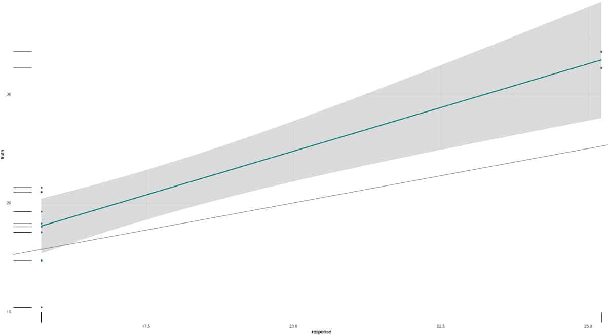
> library(mlr3viz)

> predict = learning$predict(task_mtcars, row_ids = subset$test)

> autoplot(predict)
You are encouraged to read the mlr3 package reference manual to learn more about functions, arguments and usage.


