


In this series on SageMath, we continue to explore graphs. The focus in this second article is on undirected simple graphs.
In the first article in this series on SageMath, we discussed the different ways to install and use SageMath in our systems. We also covered a few simple examples for SageMath. Please remember that SageMath uses Python 3 syntax. Except for one short snippet of code, we dealt with verbatim Python code throughout. However, by the end of the article, we had used just two lines of pure SageMath code, demonstrating why SageMath has a competitive edge over Python in scientific computing. Those two lines enabled us to draw a particular type of graph called an icosahedral graph. We concluded our discussion with the promise to continue exploring graphs in the upcoming articles in this series on SageMath. Let us begin by doing precisely that.
Over the years, Wikipedia has become an independent tutorial for many topics on science and technology. So, please refer to the Wikipedia article on graph theory for a formal treatment of the subject. If you want to learn graph theory in more detail, I recommend a textbook titled ‘Introduction to Graph Theory’ by Douglas B. West. However, my treatment of graph theory will be pretty informal.
Consider a practical example to understand how graphs help us model real-world problems. Picture a group of six people: Amrita, Biju, Chitra, Dev, Ekta, and Farhan sharing a table at a function. Some of these people are friends, while others are unknown to each other. We can represent their familiarity with each other using a graph. Consider the graph shown in Figure 1. We call this Graph_1 for ease of reference during explanations.
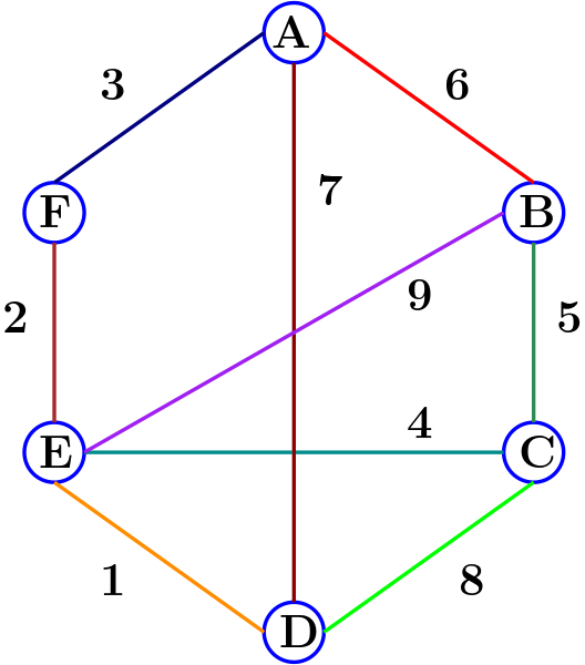
The circles in the graph are called vertices, nodes, or points. They represent the objects under discussion, in this case, the six people attending the party. The six people, Amrita, Biju, Chitra, Dev, Ekta, and Farhan, are represented by vertices labelled with upper case letters A to F, respectively. The lines connecting the vertices are called edges. In this case, the edges are used to denote whether two people are friends or not. For example, from Figure 1, it can be observed that Dev is friends with Amrita, Chitra, and Ekta but not with Biju and Farhan. The edges of a graph can also have labels or numerical weights. In Figure 1, the edge weights denote the number of years two people have been friends. For example, Dev and Chitra have been friends for eight years, whereas Dev and Ekta have been friends for just one year.
Now, let us delve into the process of creating this graph (Graph_1) using SageMath. Take a look at the SageMath code, saved as graph1.sagews, provided below (line numbers have been included for clarity in the explanation).
1. from sage.graphs.graph import Graph

2.	adj_list = {
	    “A”: {“B”: 6, “D”: 7, “F”: 3},
	    “B”: {“A”: 6, “C”: 5, “E”: 9},
	    “C”: {“B”: 5, “D”: 8, “E”: 4},
	    “D”: {“A”: 7, “C”: 8, “E”: 1},
	    “E”: {“B”: 9, “C”: 4, “D”: 1, “F”: 2},
	    “F”: {“A”: 3, “E”: 2}
	}

3.	sgraph = Graph(adj_list, weighted=True)

4.	sgraph.show(edge_labels=True)
Now, let us go through the code line by line to understand how it works. Line 1 imports the Graph class from the sage.graphs.graph module. This class is used to create and work with graph objects in SageMath. Line 2 defines an adjacency list. This line creates a Python dictionary called adj_list that represents the structure of a weighted graph. The structure of the dictionary is as follows: the keys are the vertex labels like ‘A’, ‘B’, ‘C’, etc, and the values are dictionaries containing adjacent vertices and their corresponding edge weights. For example, “A”: {“B”: 6, “D”: 7, “F”: 3} means vertex A is connected to vertices B, D, and F with weights 6, 7, and 3, respectively. Line 3 creates a weighted graph called sgraph using the Graph class. The adjacency list adj_list is given as a parameter to construct the graph. The parameter weighted is set to True to specify that the graph is weighted, meaning edges have numerical values associated with them. Finally, Line 4 displays a visual representation of the graph sgraph. The parameter edge_labels is set to True to include edge weights as labels on the edges.
Now, let us execute the code to view the output. In the first article in this series, we explored three different ways to execute SageMath code. We have decided to use an online tool called CoCalc in the initial articles in this series, so that new users can immediately start using SageMath without any installation. Log in to the CoCalc platform, type the code in the window, and save it as graph1.sagews. Now, press the Run button to execute the code. Figure 2 shows the graph generated by the above code on execution.
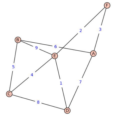
Now, here is a surprise. Compare Figures 1 and 2; they don’t look the same. I promised to generate Graph_1 (as shown in Figure 1) using SageMath, and the graph obtained (as shown in Figure 2) looks different. What happened? Well, this is an important aspect of graphs. The same graph can be drawn or embedded in different ways on paper. Thus, the two graphs in Figures 1 and 2 are equivalent; more technically, these two graphs are isomorphic, even though they look different on paper. However, the essential properties of these two graphs are the same. They have the same set of vertices, the same number of edges, and the edges connect the same pair of vertices. Furthermore, the edge weights also remain the same. For example, the edge connecting vertices A and B has a weight of 6 in both representations.
I encourage you to take some time to verify that the two representations of the graph have the same number of vertices, edges, connectivity, and weights. For a further illustration of this fact, check the Wikipedia article on the Petersen graph. The Petersen graph, comprising 10 vertices and 15 edges, is a well-known example in graph theory that illustrates how a single graph can be visually represented in various ways. Despite having the same underlying structure, different drawings or embeddings can highlight distinct features. Whether it is presented in a circular arrangement, a star-like pattern, or any other layout, the connectivity and relationships among vertices remain constant for the Petersen graph.
Recall that the above code creates a weighted graph object in SageMath using an adjacency list representation. However, this is not the only way to represent graphs in SageMath (or, for that matter, in general). One such method is to use an adjacency matrix (a grid of numbers). Add the following line of code at the end of graph1.sagews and execute it again.
print(sgraph.adjacency_matrix( ))
On execution, the following additional output will be printed on the screen. But what does it mean?
[0 1 0 1 0 1]
[1 0 1 0 1 0]
[0 1 0 1 1 0]
[1 0 1 0 1 0]
[0 1 1 1 0 1]
[1 0 0 0 1 0]
Figure 3 will help us understand the working of an adjacency matrix. An adjacency matrix is a matrix in which the rows and columns correspond to the vertices of the graph. For Graph_1, the vertices are A to F, corresponding to the six people Amrita, Biju, Chitra, Dev, Ekta, and Farhan; hence the 6 x 6 matrix. An adjacency matrix has an entry of 1 in the corresponding cell where a row and column intersect if and only if there is an edge between the pair of vertices in that particular row and column. In our example, the adjacency matrix has an entry of 1 if and only if two people are friends. For example, the cell intersecting row B and column C has an entry of 1 because Biju and Chitra are friends (please verify this from Figure 1).
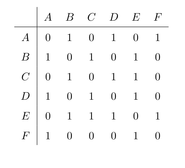
Now, consider the first row in the matrix given by Figure 3. What information do we get from it? We can see that there is no edge from vertex A to itself (this does not mean that Amrita is not friends with herself; this is just the convention I used for this example), hence the first entry is 0. The second entry is 1 because Amrita and Biju are friends. The third entry is 0 because Amrita and Chitra are not friends. The fourth entry is 1 because Amrita and Dev are friends. The fifth entry is 0 because Amrita and Ekta are not friends. The sixth entry is 1 because Amrita and Farhan are friends. Do verify these statements by looking at Figure 1, as understanding the adjacency matrix is very critical in working with graphs.
There is yet another way to represent graphs called an incidence matrix, which we will explore later in this article when discussing unweighted graphs with labels for edges.
The graph shown in Figure 1 (Graph_1) is an example of an undirected simple graph. A simple graph doesn’t contain parallel edges or loops. Parallel edges are two or more edges having the same endpoints. A loop is an edge that starts and ends at the same vertex. For example, if you want to explicitly show that Amrita is friends with herself, use an edge that starts and ends at vertex A. A graph is undirected if it only contains undirected edges. An undirected edge in a graph is like a two-way connection between two points. Think of our graph that represents friendships among people. If there’s an undirected edge between two individuals, it means they are friends, and the friendship goes both ways. It is like saying if Amrita is friends with Dev, then at the same time, Dev is friends with Amrita. The connection is reciprocal, similar to a two-way friendship on social networking sites such as Facebook. It is important to distinguish this from platforms like Instagram, where you may follow a celebrity who may not reciprocally follow you back.
Now that we have a graph depicting the relationship status of six people, what possibilities does it open up for exploration or analysis? Well, once a real-world problem is modelled as a graph, a rich set of graph-theoretic tools can be employed to extract information from the graph. It is worth noting that graph theory is a very old branch of mathematics, and its origins can be traced back to the famous problem called the Seven Bridges of Königsberg and its resolution (in the negative) by the great mathematician Leonhard Euler in 1736.
Let us look at an example of using graph theory to solve a simple problem related to the six people. Suppose we need to identify the largest group of people among these six individuals who are friends with everyone else in this group. To find a solution to this problem, add the following lines of code at the end of graph1.sagews and execute it again.
friends = sgraph.cliques_maximum( )
print(“The largest group of people who are friends with each other: “, friends)
On execution, the following additional output will be printed on the screen. But what does it mean?
The largest group of people who are friends with each other: [[‘C’, ‘E’, ‘B’], [‘D’, ‘C’, ‘E’]]
The output indicates that Biju, Chitra, and Ekta form a group of three friends, and similarly, Chitra, Dev, and Ekta constitute another group of three friends. Moreover, it can be confirmed from the graph Graph_1 that there is no group of size 4 where all four individuals are friends with each other. Solving a real-world problem was possible because we viewed it in terms of a graph-theoretic problem known as the clique problem. Formally, the clique problem is the computational problem of finding complete subgraphs in a graph. Please note that efficiently solving the clique problem is a well-known challenge in computer science. It falls into a category of problems referred to as NP-complete.
The power of a graph also derives from the fact that the same simple structure can easily abstract a lot of complicated real-world scenarios. For example, the vertices (A to F) in Graph_1 could represent places in a city. Furthermore, the edges could signify the presence of a road connecting two places, and the weight of an edge could indicate the length of the road in kilometres. With one swift stroke, the graph denoting the relationship between people transforms into the graph of a city street map. Indeed, this exemplifies the beauty and power of graph theory. Graph theory provides us with many tools to measure distances and connectivity in graphs, many of which will be explored in the upcoming articles in this series.
In a graph, the edges may not always have weights. Moreover, it is possible to assign labels to edges, similar to the labels given to vertices. Now, let us create such a graph (for ease of reference, we call it Graph_2) using SageMath. Take a look at the SageMath code saved as graph2.sagews, provided below (line numbers have been included for clarity in the explanation).
1.	from sage.graphs.graph import Graph

2.	edge_labels = {(“A”, “B”): “a”, (“B”, “C”): “b”, (“C”, “D”): “c”,
(“D”, “E”):

“d”, (“E”, “A”): “e”, (“E”, “C”): “f”}

3.	adj_list = {
	    “A”: [“B”],
	    “B”: [“C”],
	    “C”: [“D”, “E”],
	    “D”: [“E”],
	    “E”: [“A”, “C”],
	}

4.	sgraph = Graph(adj_list)

5.	for edge, label in edge_labels.items( ):
	    sgraph.set_edge_label(edge[0], edge[1], label)

6.	sgraph.show(edge_labels=True)
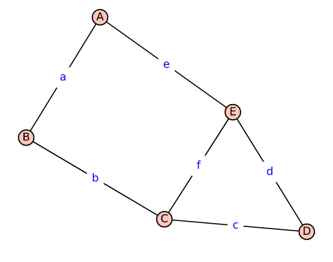
Now, let us go through the code line by line to understand its workings. In Line 1, similar to the previous program, the Graph class from the sage.graphs.graph module is imported. Line 2 creates a dictionary called edge_labels to store labels for the edges in the graph. Each key-value pair in this line represents an edge and its corresponding label. For example, (“A”, “B”): “a” means that the edge connecting vertices A and B will have the label “a”. Line 3 creates an adjacency list representation of the graph. It is a dictionary where each key is a vertex, and its value is a list of vertices that are connected to it. For example, “A”: [“B”] means that vertex A is connected to vertex B. Notice that edges are not given weights in this example. Line 4 creates a new graph object called sgraph using the adjacency list defined in adj_list. This constructs the actual graph structure in SageMath. Line 5 has a loop that iterates through the dictionary edge_labels to set the labels for each edge in the graph. The body of the loop uses the set_edge_label( ) method of the sgraph object to assign the label to the corresponding edge. Finally, Line 6 displays a visual representation of the graph sgraph. The parameter edge_labels=True ensures that the labels defined in edge_labels are displayed along with the edges while the graph is visualised. Use CoCalc to execute this code, and upon execution, the graph shown in Figure 4, called Graph_2, is obtained.
As mentioned earlier, a graph can also be represented using an incidence matrix. Now, let us examine the incidence matrix representation of the graph Graph_2. Add the following line of code at the end of graph2.sagews and execute it again.
print(sgraph.incidence_matrix( ))
On execution, the following additional output will be printed on the screen. But what does it mean?
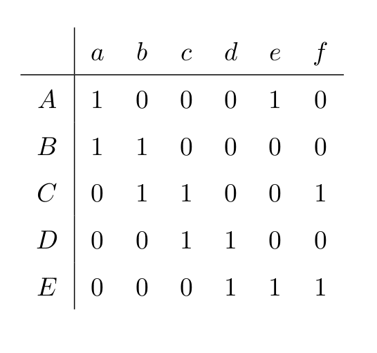
[1 1 1 0 0 0]
[1 0 0 1 0 0]
[0 1 0 1 1 0]
[0 0 1 0 0 1]
[0 0 0 0 1 1]
Figure 5 will help us understand the working of an incidence matrix. An incidence matrix is a matrix where each row represents a vertex and each column represents an edge. For Graph_2, the vertices are A to E and the edges are from a to f (hence, the 5 X 6 matrix). If a vertex is connected to an edge, then the cell corresponding to that row and column of the incidence matrix will have a 1 as its value. Otherwise, the cell will have a 0 as its value. Since every edge has exactly two endpoints, every column of the incidence matrix will have exactly two 1’s. In the next article in this series, we will do the reverse of what we did in this article. We will construct graphs by providing their adjacency matrix or incidence matrix.
Now, it is time to conclude our discussion. Graph theory, being almost three centuries old, has a lot of tools to offer. Hence, we will continue our exploration of the applications of graphs in the next article in this series as well. Although our discussion in this article focused on undirected simple graphs, there are other types of graphs, including directed graphs, multigraphs, mixed graphs, mixed multigraphs, and more. We will delve into these types of graphs also in the next article of this series.


