

By mastering the art of upsampling and downsampling, we not only correct skewed
datasets but also pave the way for fairer, more accurate machine learning models.
This second article in the two-part series focuses on the uses of downsampling.
In the first part of this article series, which was published in the March 2024 edition of OSFY, we learnt how to manage imbalanced datasets by using upsampling techniques. Now, let us see how downsampling works.
Downsampling
Downsampling is used to decrease the size of a dataset by removing some of the instances. When the data is imbalanced, the data points of the majority class are removed. This is often done to reduce computational complexity and training time, and to eliminate redundancy or irrelevant instances from the dataset. However, when doing this, we need to ensure important information is not lost and the sample represents the entire dataset.
Methods used in downsampling
Upsampling is used when the dataset is large. Downsampling is a good option to reduce the computational complexity and training time of the model. If the goal is to improve model efficiency or reduce the risk of overfitting, downsampling is a better option. A few methods used for downsampling are explained here, though these are not exhaustive.
Resample
- This method which is used for upsampling can be used for downsampling as well. The simplest way of downsampling majority classes is by randomly removing records from that category.
- Logic used is the same as upsampling — instead of increasing random records, remove them.
- Here is sample code:
from collections import Counter
from sklearn.datasets import make_classification
from sklearn.utils import resample
from matplotlib import pyplot
from numpy import where
import pandas as pd
import numpy as np
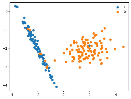
X, y = make_classification(n_classes=2, class_sep=2,
weights=[0.1, 0.9], n_features=4, n_clusters_per_class=1, n_samples=1000, random_state=10)
# summarize class distribution
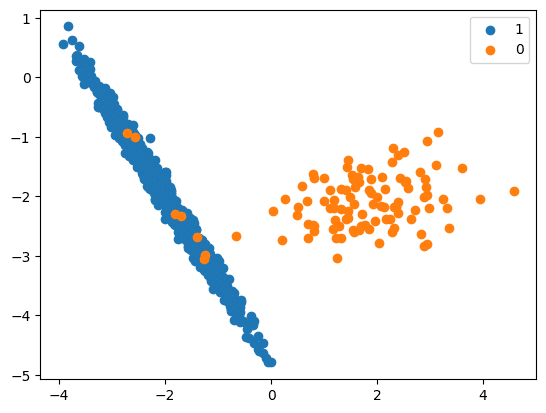
print(‘Original dataset shape %s’ % Counter(y))
Original dataset shape Counter({1: 894, 0: 106})
# scatter plot of examples by class label
for label, _ in Counter(y).items():
row_ix = where(y == label)[0]
pyplot.scatter(X[row_ix, 0], X[row_ix, 1], label=str(label))
pyplot.legend()
pyplot.show()
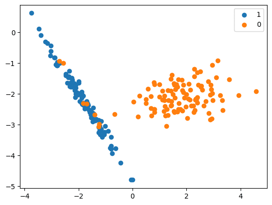
# perform downsampling
df = pd.DataFrame(X, columns=[‘Column_A’, ‘Column_B’, ‘Column_C’, ‘Column_D’])
df[‘Y’] = y
over_samples = df[df[“Y”] == 1]
under_samples = df[df[“Y”] == 0]
print(“Original Over Sample Shape”, under_samples.shape)
df_res = resample(over_samples,
replace=True,
n_samples=len(under_samples),
random_state=42)
print(“Resampled Over Sample Shape”, df_res.shape)
X_Res = np.append(df_res[[‘Column_A’, ‘Column_B’, ‘Column_C’, ‘Column_D’]].to_numpy(), under_samples[[‘Column_A’, ‘Column_B’, ‘Column_C’, ‘Column_D’]].to_numpy(), axis=0)
y_res = np.append(df_res[‘Y’].to_numpy(), under_samples[‘Y’].to_numpy())
print(‘Resampled dataset shape %s’ % Counter(y_res))
Original Over Sample Shape (106, 5)
Resampled Over Sample Shape (894, 5)
Resampled dataset shape Counter({0: 894, 1: 894})
# scatter plot of examples by class label
for label, _ in Counter(y_res).items():
row_ix = where(y_res == label)[0]
pyplot.scatter(X_Res[row_ix, 0], X_Res[row_ix, 1], label=str(label))
pyplot.legend()
pyplot.show()

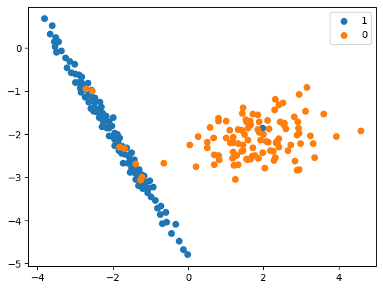
RandomUnderSampler
- In this method, the rows from the majority class are selected randomly and replaced.
- Logic used is the same as that used for upsampling, except the strategies in this case impact the majority class instead of the minority class.
- The source code is:
from collections import Counter
from sklearn.datasets import make_classification
from imblearn.under_sampling import RandomUnderSampler
from matplotlib import pyplot
from numpy import where
X, y = make_classification(n_classes=2, class_sep=2,
weights=[0.1, 0.9], n_features=4, n_clusters_per_class=1, n_samples=1000, random_state=10)
# summarize class distribution
print(‘Original dataset shape %s’ % Counter(y))
Original dataset shape Counter({1: 894, 0: 106})
Now we will carry out downsampling:
rus = RandomUnderSampler(random_state=42)
X_Res, y_res = rus.fit_resample(X, y)
print(‘Resampled dataset shape %s’ % Counter(y_res))
Resampled dataset shape Counter({0: 106, 1: 106})
# scatter plot of examples by class label
for label, _ in Counter(y_res).items():
row_ix = where(y_res == label)[0]
pyplot.scatter(X_Res[row_ix, 0], X_Res[row_ix, 1], label=str(label))
pyplot.legend()
pyplot.show()
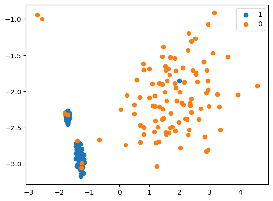
Cluster centroid
- The centroid algorithm uses the K-Means method to replace the samples under the majority class.
- This method handles the imbalanced datasets and involves undersampling the majority class by replacing a group of majority samples with the cluster centroid of a K-Means algorithm. This newly generated set is created using the centroids of the K-Means method instead of the original samples. By doing this, the majority class(es) are transformed while the minority class remains unchanged.
- The logic is:
- Choose random data from the majority class.
- Calculate the Euclidean distance between the random data and its k nearest neighbours.
- Calculate centroids for clusters and use them to represent the majority class, reducing samples.
- Repeat the procedure until the desired proportion of minority classes is met.
- The sample code is:
from collections import Counter
from sklearn.datasets import make_classification
from sklearn.utils import resample
from imblearn.under_sampling import ClusterCentroids
from sklearn.cluster import MiniBatchKMeans
from matplotlib import pyplot
from numpy import where
X, y = make_classification(n_classes=2, class_sep=2,
weights=[0.1, 0.9], n_features=4, n_clusters_per_class=1, n_samples=1000, random_state=10)
# summarize class distribution
print(‘Original dataset shape %s’ % Counter(y))
Original dataset shape Counter({1: 894, 0: 106})
Now we will carry out downsampling:
cc = ClusterCentroids(
estimator=MiniBatchKMeans(n_init=1, random_state=0), random_state=42
)
X_Res, y_res = cc.fit_resample(X, y)
print(‘Resampled dataset shape %s’ % Counter(y_res))
Resampled dataset shape Counter({0: 106, 1: 106})
# scatter plot of examples by class label
for label, _ in Counter(y_res).items():
row_ix = where(y_res == label)[0]
pyplot.scatter(X_Res[row_ix, 0], X_Res[row_ix, 1], label=str(label))
pyplot.legend()
pyplot.show()
NearMiss
- In this method, the majority class instances that are near the minority class instances are removed.
- There are three versions of this algorithm, and each version has a different criterion for selecting which majority class instances to keep and which ones to discard.
- NearMiss-1: The data is balanced by selecting the samples from the majority class for which the average distance of the k nearest samples of the minority class is the smallest.
- NearMiss-2: The data is balanced by selecting the samples from the majority class for which the average distance to the farthest samples of the minority class is the smallest.
- NearMiss-3: This is a 2-step algorithm: first, the m nearest-neighbours are kept for each minority sample; then, the majority samples for which the average distance to the k nearest neighbours is the largest are selected.
- The logic is:
- This algorithm has two important parameters — version and k neighbours.
- It calculates the distance between all the points in the larger class with the points in the smaller class.
- Elimination is done based on the passed parameter.
- NearMiss-1: This version keeps instances from the majority class that are closest to the instances in the minority class.
- NearMiss-2: This version removes instances from the majority class that are farthest from the minority class.
- NearMiss-3: This version is somewhat opposite to NearMiss-1; it keeps instances from the majority class that are farthest from the instances in the minority class.
- The sample code is:
from collections import Counter

from sklearn.datasets import make_classification

from sklearn.utils import resample

from imblearn.under_sampling import NearMiss

from matplotlib import pyplot

from numpy import where

X, y = make_classification(n_classes=2, class_sep=2,

weights=[0.1, 0.9], n_features=4, n_clusters_per_class=1, n_samples=1000, random_state=10)

# summarise class distribution

print(‘Original dataset shape %s’ % Counter(y))

Original dataset shape Counter({1: 894, 0: 106})
We will now perform downsampling:
cc = NearMiss()

X_Res, y_res = cc.fit_resample(X, y)

print(‘Resampled dataset shape %s’ % Counter(y_res))

Resampled dataset shape Counter({0: 106, 1: 106})

# scatter plot of examples by class label

for label, _ in Counter(y_res).items():

row_ix = where(y_res == label)[0]

pyplot.scatter(X_Res[row_ix, 0], X_Res[row_ix, 1], label=str(label))

pyplot.legend()

pyplot.show()
Tomek links (T-links)
- Here a pair of data points from different classes (nearest-neighbours) are dropped — the objective is to drop the sample that corresponds to the majority and thereby minimise the count of the dominating label.
- This also increases the border space between the two labels and thus enhances the accuracy of the performance.
- Here’s the logic.
- Identifying Tomek links:
- A Tomek link is a pair of instances (x, y) where x is from the majority class and y is from the minority class, leaving no other smaller instance between.
- Removing instances in Tomek links:
- Once Tomek links are identified, the instances from the majority class in these links are removed.
- This helps in creating a cleaner and more separable boundary between the classes.
- Resulting effect:
- The removal of instances involved in Tomek links can enhance the performance of a machine learning model by reducing noise in the dataset and improving the separation between classes.
- Identifying Tomek links:
- The source code is:
from collections import Counter

from sklearn.datasets import make_classification

from sklearn.utils import resample

from imblearn.under_sampling import TomekLinks

from matplotlib import pyplot

from numpy import where

X, y = make_classification(n_classes=2, class_sep=2,

weights=[0.1, 0.9], n_features=4, n_clusters_per_class=1, n_samples=1000, random_state=10)

# summarize class distribution

print(‘Original dataset shape %s’ % Counter(y))

Original dataset shape Counter({1: 894, 0: 106})
Next, we will carry out downsampling:
cc = TomekLinks()

X_Res, y_res = cc.fit_resample(X, y)

print(‘Resampled dataset shape %s’ % Counter(y_res))

Resampled dataset shape Counter({1: 890, 0: 106})

# scatter plot of examples by class label

for label, _ in Counter(y_res).items():

row_ix = where(y_res == label)[0]

pyplot.scatter(X_Res[row_ix, 0], X_Res[row_ix, 1], label=str(label))

pyplot.legend()

pyplot.show()

AIIKNN (All K-Nearest-Neighbours)
- This method works by removing some of the instances from the majority class that are considered to be ‘misclassified’ or near the decision boundary.
- The goal is to create a more balanced dataset by eliminating instances from the majority class that may be causing confusion for the classifier.
- The logic is:
-
- AllKNN is a modification of RepeatedEditedNearestNeighbours (RENN) that expands the size of the neighbourhood being considered each time it is run.
- The RENN algorithm runs the EditedNearestNeighbour (ENN) algorithm a specified number of times, removing more outlier points with each rerun.
- ENN removes misclassified instances near the decision boundary from the majority class.
- The sample code is:
from collections import Counter

from sklearn.datasets import make_classification

from sklearn.utils import resample

from imblearn.under_sampling import AllKNN

from matplotlib import pyplot

from numpy import where

X, y = make_classification(n_classes=2, class_sep=2,

weights=[0.1, 0.9], n_features=4, n_clusters_per_class=1, n_samples=1000, random_state=10)

# summarise class distribution

print(‘Original dataset shape %s’ % Counter(y))

Original dataset shape Counter({1: 894, 0: 106})

# perform downsampling

allknn = AllKNN()

X_Res, y_res = allknn.fit_resample(X, y)

print(‘Resampled dataset shape %s’ % Counter(y_res))

Resampled dataset shape Counter({1: 872, 0: 106})

# scatter plot of examples by class label

for label, _ in Counter(y_res).items():

row_ix = where(y_res == label)[0]

pyplot.scatter(X_Res[row_ix, 0], X_Res[row_ix, 1], label=str(label))

pyplot.legend()

pyplot.show()
Pros and cons of downsampling
Pros
- Helps in reducing the bias where the class is over-populated.
- Reduces noise and improves accuracy.
- Saves training time and reduces the computational power needed.
Cons
- Can result in information loss.
- Post downsampling, the remaining dataset can lead to overfitting or biased results.

To sum up, upsampling involves an increase in the minority class while downsampling is vice-versa – it involves a decrease in the majority class. These equalisation processes prevent the machine learning model from inclining towards the majority class. Remember that upsampling and downsampling need to preserve the distribution of the data, and the boundary line between the target classes must remain the same. Also, upsampling and downsampling are applied only to the training datasets and no changes are made to validation and testing data.


