
























































Quantum machine learning can appear intimidating because it combines two complex subjects. PennyLane lowers that barrier by allowing developers to write a quantum circuit as a trainable component inside a familiar Python machine-learning workflow.
Quantum machine learning brings quantum circuits into the machine-learning workflow. In present-day experiments, a classical computer still prepares the data, controls training and interprets the result, while a quantum circuit acts as a specialised trainable processing component. This combination is called hybrid quantum-classical machine learning.
The goal is not to assume that quantum models are automatically better. The immediate value is the ability to investigate new ways of representing data, combining features and solving optimisation problems using open source tools.
What is PennyLane?
PennyLane is open source and developed by Xanadu. Its documentation describes it as a platform for quantum computing, quantum machine learning and quantum chemistry. The framework currently integrates with PyTorch, JAX and PennyLane NumPy, and its device abstraction allows the same high-level circuit to run on simulators or supported hardware backends. For new machine-learning projects, the current documentation recommends PyTorch or JAX; TensorFlow support in PennyLane is no longer maintained from version 0.44 onward.
Why PennyLane is needed
A beginner entering quantum computing quickly encounters Qiskit, Cirq, TensorFlow Quantum, Q#, pyQuil, and several hardware-specific tools. All of them can describe quantum programs, but they were not created around the same question. Some concentrate on building and compiling circuits for a particular hardware ecosystem. Others focus on hardware research, simulation, or a programming language. PennyLane places a different question at the centre: how can a quantum circuit be trained together with an ordinary machine learning model?
That distinction matters. In a conventional neural network, a framework such as PyTorch keeps track of operations, calculates gradients, and adjusts weights. PennyLane extends this style of differentiable programming to quantum circuits. A circuit can receive data, expose trainable gate parameters, return measurements and participate in the same optimisation loop as a classical layer.
How PennyLane works
PennyLane receives classical input values, uses them to control quantum gates, executes a circuit on a selected device, measures the resulting qubit states and returns ordinary numerical values. Those values can then be used by PyTorch or JAX to calculate a prediction and train the complete model.
A PennyLane program has four important parts:
- Device: The simulator or quantum processor on which the circuit executes.
- Quantum function: The sequence of gates applied to named qubits, called wires in PennyLane.
- QNode: A wrapper that connects the quantum function to a device and to an automatic-differentiation interface.
- Optimizer or ML framework: PyTorch, JAX or another supported interface that updates trainable parameters.
The QNode is the key bridge. From the machine learning side it behaves like a numerical function or layer. Internally, it prepares qubits, applies gates, executes the circuit, and returns measurement values. PennyLane then determines how those values change when the circuit parameters change.
The hybrid processing path
Consider two Iris measurements: petal length and petal width. After preprocessing, each value controls a rotation gate on one qubit. The rotations do not place decimal centimetre values into qubits as binary digits. Instead, each value tells the circuit how far to change a qubit’s state. Additional rotations contain trainable parameters, and an entangling gate allows the two qubits to interact. Finally, the circuit measures the qubits and returns ordinary numbers. A small classical layer converts those numbers into a class probability as shown in Figure 1.
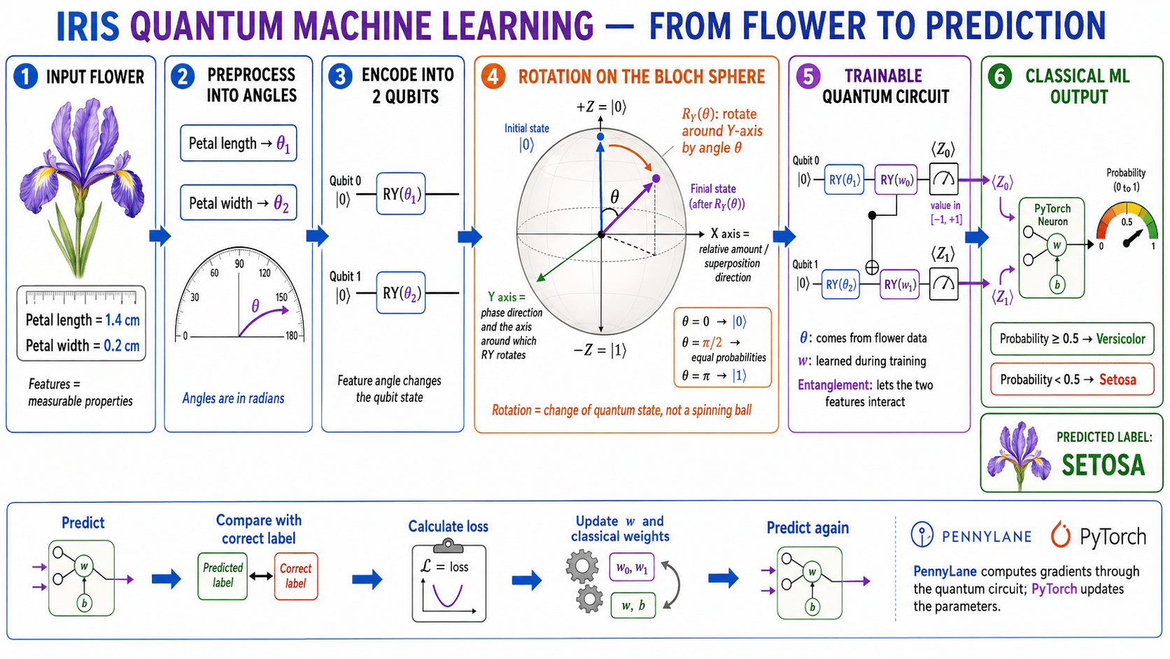
Training repeatedly follows the same loop: encode a flower, run the circuit, measure it, predict a class, compare the prediction with the known label, calculate the error, and update both the quantum and classical parameters. This is a hybrid model because the quantum circuit supplies a trainable transformation while the classical computer handles data preparation, optimisation and the final decision.
Major strengths of PennyLane
Differentiable quantum programming
PennyLane’s defining strength is gradient-based training across quantum and classical operations. Developers can place a circuit inside a PyTorch module and allow the optimiser to update circuit angles alongside ordinary neural-network weights. This makes small quantum neural networks and variational algorithms comparatively natural to prototype.
Backend flexibility
The device interface separates the circuit description from its execution backend. A learner can begin with the built-in default.qubit simulator and later experiment with a plugin for another simulator or supported provider. Hardware portability is never completely automatic—devices differ in gates, connectivity, noise and execution rules—but the abstraction reduces the amount of application code tied to one vendor.
Familiar Python and ML integration
PennyLane deliberately feels close to scientific Python. Quantum gates are written as Python operations, measurements are returned like numerical outputs, and QNodes can accept PyTorch tensors or JAX arrays. This is especially helpful for ML practitioners who want to learn quantum circuits without abandoning their existing optimisation workflow.
A strong educational and research workflow
The framework can draw circuits, inspect operations, simulate ideal or noisy execution and calculate gradients without requiring access to physical hardware. It is therefore useful in classrooms, notebooks, and early-stage research, where understanding the model is more important than immediately deploying it on a quantum processor.
A comparison with other quantum frameworks
No framework is universally best. The useful comparison is not whether one can create a circuit—they all can—but which workflow receives first-class attention (Table 1).
| Framework | Primary emphasis | ML integration | Hardware orientation | Natural choice when… |
| PennyLane | Differentiable quantum and hybrid programming | Strong PyTorch/JAX integration | Multi-backend through devices and plugins | The quantum circuit must behave like a trainable ML layer |
| Qiskit | Broad quantum workflows, compilation and execution | QML is available within a wider ecosystem | Strong IBM Quantum integration | You need IBM hardware, transpilation or general quantum development |
| Cirq | Circuit construction, manipulation and NISQ hardware detail | Possible directly or through other libraries | Hardware-aware, especially Google-oriented research | You need fine circuit and device control |
| TensorFlow Quantum | Hybrid QML inside TensorFlow using Cirq | Native TensorFlow/Keras workflow | Cirq-based execution model | Your project is already centred on TensorFlow and Cirq |
| Q# | Quantum algorithm expression and resource reasoning | Not primarily an ML-layer framework | Microsoft/Azure quantum ecosystem | You want a dedicated quantum language or resource estimation |
Table 1: Framework choice should follow the intended workflow rather than brand popularity
Qiskit is broader than PennyLane and is the natural entry point to IBM’s ecosystem. Cirq exposes circuit and device details suited to NISQ experiments. TensorFlow Quantum builds hybrid models by bringing Cirq circuits into TensorFlow. PennyLane is particularly attractive when the central requirement is end-to-end optimisation of a quantum circuit together with classical ML components.
Important use cases of PennyLane are:
- Quantum neural networks for classification and regression experiments.
- Variational quantum algorithms in which gate parameters are iteratively optimised.
- Quantum kernels and feature maps for exploring alternative representations of data.
- Quantum chemistry, including molecular Hamiltonians and variational energy estimation.
- Combinatorial optimisation prototypes using hybrid objective functions.
- Generative and probabilistic quantum models.
- Education, circuit visualisation, gradient demonstrations and backend comparison.
These are research and experimentation use cases. Present-day QML should not be presented as a guaranteed replacement for classical machine learning. Small demonstrations are valuable for learning the workflow and evaluating hypotheses, but performance, noise, data-loading cost, and fair classical baselines remain essential considerations.
The Iris dataset experiment
The Iris dataset contains 150 samples, four numerical measurements and three flower species. To keep the first experiment easy to inspect, we use 100 samples from two species—Setosa and Versicolor—and two features: petal length and petal width. Seventy-five samples are used for training and 25 for testing. One feature is angle-encoded on each of the two qubits.
The circuit uses feature rotations, two trainable entangling layers and measurements from both qubits. PennyLane converts the circuit into a PyTorch layer. A classical linear layer and sigmoid output then produce the Versicolor probability.
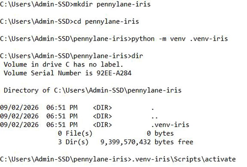
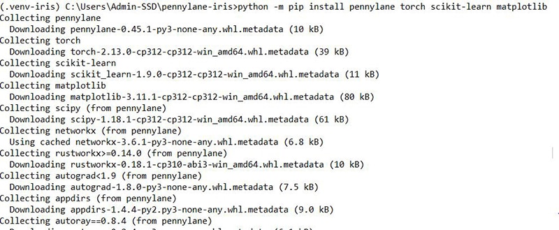
The setup begins by creating and activating a dedicated Python virtual environment, which keeps the experiment and its dependencies isolated from other projects as shown in Figure 2. PennyLane, PyTorch, Scikit-learn and Matplotlib are then installed using pip as shown in Figure 3. These libraries provide the tools required for quantum-circuit construction, model training, dataset preparation, and result visualisation.
Preparing the Iris dataset
The program loads Iris from Scikit-learn, keeps Setosa and Versicolor, selects petal length and petal width, and divides the data into stratified training and test sets. Standardisation places both features on a comparable scale.
Encoding flower features into qubits
After preprocessing, petal length controls the rotation of Qubit 0 and petal width controls the rotation of Qubit 1. Different flowers therefore create different qubit states. The values are used as rotation instructions rather than being stored in the qubits as ordinary binary numbers.
Building the quantum circuit
The circuit first performs feature encoding, then applies trainable rotations and entanglement. Entanglement allows the circuit to process the relationship between the two flower measurements. Finally, both qubits are measured to produce two ordinary numerical outputs.
Connecting PennyLane with PyTorch
PennyLane’s TorchLayer converts the QNode into a PyTorch-compatible layer. A classical linear layer receives the two quantum measurements, and a sigmoid output converts them into the probability of the flower being Versicolor.
Training the hybrid QML model
For every epoch, the model processes all training flowers, calculates prediction loss, and uses the Adam optimiser to update both the trainable quantum angles and the classical layer parameters. PennyLane supplies gradients through the circuit while PyTorch manages the optimisation loop.
Here’s the complete Python Program:
import numpy as np

import pennylane as qml

import torch

from torch import nn

from sklearn.datasets import load_iris

from sklearn.model_selection import train_test_split

from sklearn.preprocessing import StandardScaler

from sklearn.metrics import accuracy_score, confusion_matrix

SEED = 42

np.random.seed(SEED)

torch.manual_seed(SEED)

# 1. Load two classes and two petal features

iris = load_iris()

keep = iris.target < 2

X = iris.data[keep][:, [2, 3]]

y = iris.target[keep]

X_train, X_test, y_train, y_test = train_test_split(

X, y, test_size=0.25, random_state=SEED, stratify=y

)

# 2. Scale the data, then bound it into convenient angles

scaler = StandardScaler()

X_train = np.arctan(scaler.fit_transform(X_train))

X_test = np.arctan(scaler.transform(X_test))

X_train = torch.tensor(X_train, dtype=torch.float32)

X_test = torch.tensor(X_test, dtype=torch.float32)

y_train = torch.tensor(y_train, dtype=torch.float32).reshape(-1, 1)

y_test = torch.tensor(y_test, dtype=torch.float32).reshape(-1, 1)

# 3. Create a two-qubit simulator

dev = qml.device(“default.qubit”, wires=2)

# 4. Define the trainable quantum circuit

@qml.qnode(dev, interface=”torch”, diff_method=”backprop”)

def circuit(inputs, weights):

qml.AngleEmbedding(inputs, wires=[0, 1], rotation=”Y”)

qml.BasicEntanglerLayers(weights, wires=[0, 1])

return [qml.expval(qml.PauliZ(w)) for w in [0, 1]]

# 5. Convert the QNode into a PyTorch layer

quantum_layer = qml.qnn.TorchLayer(

circuit, {“weights”: (2, 2)}

)

model = nn.Sequential(

quantum_layer,

nn.Linear(2, 1),

nn.Sigmoid()

)

# 6. Train quantum and classical parameters together

loss_fn = nn.BCELoss()

optimizer = torch.optim.Adam(model.parameters(), lr=0.05)

for epoch in range(1, 51):

optimizer.zero_grad()

probability = model(X_train)

loss = loss_fn(probability, y_train)

loss.backward()

optimizer.step()

if epoch == 1 or epoch % 10 == 0:

pred = (probability >= 0.5).int().numpy().ravel()

acc = accuracy_score(y_train.numpy().ravel(), pred)

print(f”Epoch {epoch:02d}: loss={loss.item():.4f}, “

f”training accuracy={acc:.3f}”)

# 7. Evaluate unseen test flowers

model.eval()

with torch.no_grad():

probability = model(X_test)

prediction = (probability >= 0.5).int().numpy().ravel()

truth = y_test.int().numpy().ravel()

print(“Test accuracy:”, accuracy_score(truth, prediction))

print(“Confusion matrix:\n”, confusion_matrix(truth, prediction))
Understanding the code without quantum mathematics
The data section selects only Setosa and Versicolor, and keeps petal length and width. Standardisation prevents the two measurements from being treated on incompatible scales. The arctangent bounds the transformed values so they remain convenient rotation inputs.
The device named default.qubit is a simulator, so no physical quantum computer or cloud account is required. AngleEmbedding rotates the two qubits according to the two flower features. BasicEntanglerLayers supplies trainable rotations and an interaction between qubits. The two measurements returned by the QNode become two ordinary numbers.
TorchLayer packages the QNode as a PyTorch module. From this point onwards, PyTorch can place the quantum layer inside a sequential model, calculate binary cross-entropy loss and update all trainable parameters with Adam. The developer does not need to create a separate optimisation routine for the quantum part.
| Experiment setting | Observed value |
| Training/test samples | 75 / 25 |
| Qubits | 2 |
| Epochs | 50 |
| Final training loss | 0.1058 |
| Test accuracy | 100% (25/25) |
| Confusion matrix | 13 Setosa correct; 12 Versicolor correct; 0 errors |
Table 2: Reproducible result obtained with the listed split, seed and training configuration
Experimental results
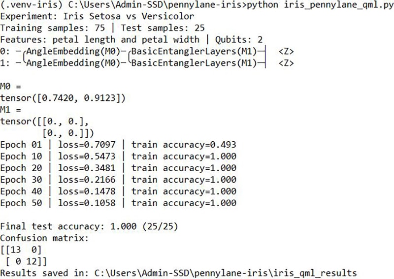
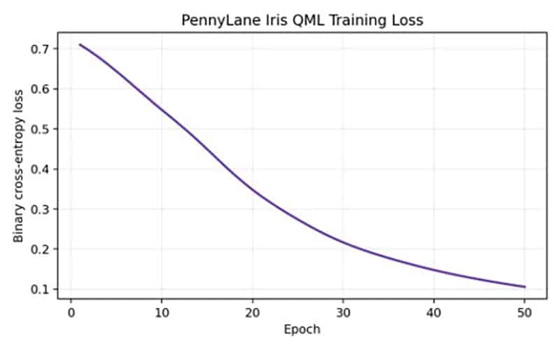
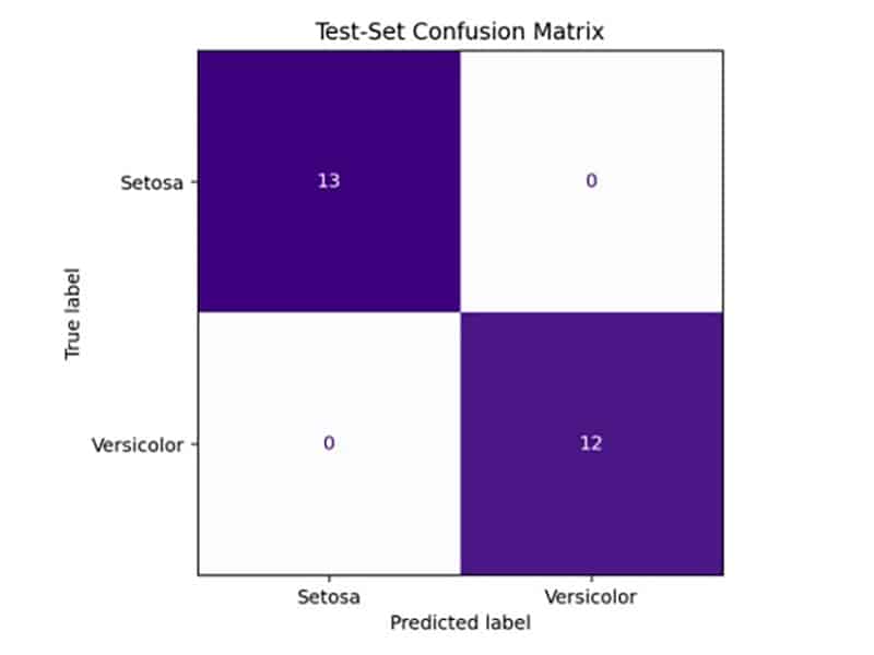
With the fixed random seed and the stated 75/25 stratified split, the training loss fell from 0.7097 in the first epoch to 0.1058 after 50 epochs. Training accuracy reached 100 per cent by epoch 10. On the held-out test set, all 25 flowers were classified correctly: 13 Setosa and 12 Versicolor as shown in Figure 4.
Understanding the results
This trained model correctly classified all 25 test flowers in this split as shown in Figure 5. This does not mean that PennyLane always produces perfect models, that every Iris split will produce the same result, or that quantum computing has outperformed classical machine learning. Setosa and Versicolor are easily separated using petal measurements, and classical models can also solve this small task very well.
The value of this experiment is educational: it exposes every stage of a hybrid QML workflow in a problem that runs quickly on a laptop. A serious comparison would require repeated splits, multiple random seeds, classical baselines, noise experiments, runtime and resource measurements, and preferably a problem for which the quantum representation has a defensible motivation.
Limitations of the experiment
Quantum simulators become expensive as the qubit count increases because a general state-vector simulation grows exponentially. Physical quantum processors introduce noise, restricted qubit connectivity, queueing and finite measurement shots. Classical data must also be encoded into the circuit, and that cost can outweigh any benefit if the representation is not chosen carefully.
Hybrid QML is therefore an active research area rather than a drop-in performance upgrade. PennyLane’s strength is that it makes controlled experimentation easier: the same conceptual model can be studied with multiple differentiation techniques, simulators, noise models and supported backends while remaining connected to familiar ML tooling.
Possible extensions are:
- Include Virginica and replace the binary output with a three-class classifier.
- Encode all four Iris features using four qubits or a data re-uploading circuit.
- Compare different embeddings, entanglement patterns and circuit depths.
- Add simulated noise and study whether accuracy and convergence change.
- Compare the hybrid model with logistic regression, SVM and a small classical neural network.
- Execute a suitably compiled version on an accessible hardware backend and compare it with ideal simulation.
- Use repeated train/test splits and report average accuracy with variability, not only one split.
PennyLane occupies a clear position in the open source quantum ecosystem. Qiskit offers a broad IBM-centred development and execution environment; Cirq provides strong circuit and NISQ-device abstractions; TensorFlow Quantum integrates Cirq with TensorFlow. PennyLane distinguishes itself by treating differentiable quantum circuits as trainable building blocks within hybrid applications.
For a newcomer to QML, that design provides a gentle and productive path: begin on a simulator, encode a small dataset, build a shallow circuit, connect it to PyTorch, observe the training loop and only then explore deeper circuits, noise and hardware. The Iris example does not demonstrate quantum advantage, but shows something equally important for a beginner—the complete route from classical data to qubits and back to a usable prediction.