
In the simplest of terms, a neural network is a computer system modelled on the human nervous system. It is widely used in machine learning technology. R is an open source programming language, which is mostly used by statisticians and data miners. It greatly supports machine learning, for which it has many packages.
The neural network is the most widely used machine learning technology available today. Its algorithm mimics the functioning of the human brain to train a computational network to identify the inherent patterns of the data under investigation. There are several variations of this computational network to process data, but the most common is the feedforward-backpropagation configuration. Many tools are available for its implementation, but most of them are expensive and proprietary. There are at least 30 different packages of open source neural network software available, and of them, R, with its rich neural network packages, is much ahead.
R provides this machine learning environment under a strong programming platform, which not only provides the supporting computation paradigm but also offers enormous flexibility on related data processing. The open source version of R and the supporting neural network packages are very easy to install and also comparatively simple to learn. In this article, I will demonstrate machine learning using a neural network to solve quadratic equation problems. I have chosen a simple problem as an example, to help you learn machine learning concepts and understand the training procedure of a neural network. Machine learning is widely used in many areas, ranging from the diagnosis of diseases to weather forecasting. You can also experiment with any novel example, which you feel can be interesting to solve using a neural network.
Quadratic equations
The example I have chosen shows how to train a neural network model to solve a set of quadratic equations. The general form of a quadratic equation is: ax2 + bx + c = 0. At the outset, let us consider three sets of coefficients a, b and c and calculate the corresponding roots r1 and r2.
The coefficients are processed to eliminate the linear equations with negative values of the discriminant, i.e., when b2 – 4ac < 0. A neural network is then trained with these data sets. Coefficients and roots are numerical vectors, and they have been converted to the data frame for further operations.
The example of training data sets consists of three coefficients with 10 values each:
aa<-c(1, 1, -3, 1, -5, 2,2,2,1,1)

bb<-c(5, -3, -1, 10, 7, -7,1,1,-4,-25)

cc<-c(6, -10, -1, 24, 9, 3,-4,4,-21,156)
Data preprocessing
To discard equations with zero as coefficients of x2, use the following code:
k <- which(aa != 0)

aa <-aa[k]

bb <-bb[k]

cc <-cc[k]
To accept only those coefficients for which the discriminant is zero or more, use the code given below:
disc <-(bb*bb-4*aa*cc)

k <- which(disc >= 0)

aa <-aa[k]

bb <-bb[k]

cc <-cc[k]

a <- as.data.frame(aa) # a,b,c vectors are converted to data frame

b <- as.data.frame(bb)

c <- as.data.frame(cc)
Calculate the roots of valid equations using conventional formulae, for training and verification of the machine’s results at a later stage.
r1 <- (-b + sqrt(b*b-4*a*c))/(2*a) # r1 and r2 roots of each equations

r2 <- (-b - sqrt(b*b-4*a*c))/(2*a)
After getting all the coefficients and roots of the equations, concatenate them columnwise to form the input-output data sets of a neural network.
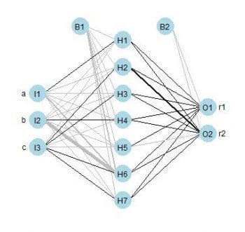
Since this is a simple problem, the network is configured with three nodes in the input-layer, one hidden-layer with seven nodes and a two-node output-layer.
R function neuralnet() requires input-output data in a proper format. The format of formulation procedure is somewhat tricky and requires attention. The right hand side of the formula consists of two roots and the left side includes three coefficients a, b and c. The inclusion is represented by + signs.
colnames(trainingdata) <- c(“a”,”b”,”c”,”r1”,”r2”)

net.quadroot <- neuralnet(r1+r2~a+b+c, trainingdata, hidden=7, threshold=0.0001)
An arbitrary performance threshold value 10-4 is taken and this can be adjusted as per requirements.
The configuration of the just-constructed model with its training data can be visualised with a plot function.
#Plot the neural network

plot(net.quadroot)
Now it is time to verify the neural net with a set of unknown data. Arbitrarily take a few sets of values of three coefficients for the corresponding quadratic equations, and arrange them as data frames as shown below.
x1<-c(1, 1, 1, -2, 1, 2)

x2<-c(5, 4, -2, -1, 9, 1)

x3<-c(6, 5, -8, -2, 22, -3)
Since there is no zero coefficient corresponding to x2, we can accept only those coefficients for which the discriminant is zero or more than zero.
disc <-(x2*x2-4*x1*x3)

k <- which(disc >= 0)

x1 <-x1[k]

x2 <-x2[k]

x3 <-x3[k]

y1=as.data.frame(x1)

y2=as.data.frame(x2)

y3=as.data.frame(x3)
The values are then fed to the just-configured neural model net.quadroot to predict their roots. The predicted roots are collected into net.result$net.result and can be displayed with the print() function.
testdata <- cbind(y1,y2,y3)

net.results <- compute(net.quadroot, testdata)

#Lets see the results

print(net.results$net.result)
Now, how does one verify the results? To do this, let us compute the roots using the conventional root calculation formula, and verify the results by comparing the predicted values with them.
Calculate the roots and concatenate them into a data frame.
calr1 <- (-y2 + sqrt(y2*y2-4*y1*y3))/(2*y1)

calr2 <- (-y2 - sqrt(y2*y2-4*y1*y3))/(2*y1)

r<-cbind(calr1,calr2) #Calculated roots using formula
Then combine the test data, its roots and the predicted roots into a data frame for a decent tabular display for verification (Table 1).
#Combine Inputs, Expected roots and predicted roots.

comboutput <- cbind(testdata,r,net.results$net.result)

#Put some appropriate column heading

colnames(comboutput) <- c(“a”,”b”,”c”,”r1”,”r2”,”pre-r1”,”pre-r2”)

print(comboutput)
It is clear from the above outputs that our neural network has learnt appropriately and produces an almost correct result. You may need to run the neural network several times with the given parameters to achieve a correct result. But if you are lucky, you may get the right result in the first attempt itself!


