


In the previous article in this series on AI and machine learning, we began by exploring the intricacies of using TensorFlow, a very powerful library used for developing AI and machine learning applications. Then, we discussed probability and paved the way for many of our future discussions. In this article, the fifth in the series, we will continue exploring concepts in probability and statistics.
To begin with, let us first install Anaconda, a distribution of Python for scientific computing especially useful for developing AI, machine learning and data science based applications. Later, we will also introduce a Python library called Theano in the context of probability theory. But before doing that, let us discuss the future of AI a little bit.
While going through the earlier articles in this series for evaluation and course correction, I wondered whether my tone was a bit sceptical at times while discussing the future of AI. By being brutally honest about some of the topics we discussed, I may have inadvertently demotivated a tiny fraction of the readers and potential practitioners of AI.
This made me research the financial aspects of AI and machine learning. I wanted to identify the kind of companies involved in the AI market. Are the bigwigs heavily involved or are there just some startups trying to move away from the pack? Another important question was: how much money will be pumped into the AI market by these companies in the near future? Is it going to be just a couple of million, or a few billion or maybe even a few trillion?
For the predictions and data stated here, I depended on articles published in respected newspapers in the recent past rather than on scholarly articles which I couldn’t grasp well to understand the complex dynamics behind the development of an AI based economy. An article published by Forbes in had 2020 predicted that companies would spend 50 billion dollars on AI in financial year 2020. Well, that is a really huge investment, even if we acknowledge that the American billion (109) is just one-thousandth of the British billion (1012). An article published in Fortune, another American business magazine, reported that venture capitalists are shifting some of their focus from artificial intelligence to newer and trendier fields like Web3 and decentralised finance (DeFi). But The Wall Street Journal (an American business-focused newspaper) in 2022 confidently predicted that, ‘Big Tech Is Spending Billions on AI Research. Investors Should Keep an Eye Out’.
What about the Indian scenario? Business Standard reported in 2022 that 87 per cent of the Indian companies will hike their AI expenditure by 10 per cent in the next three years. So, overall, it looks like the future of AI is very safe and bright. But which are the top companies investing in AI? As expected, all the giants like Amazon, Meta (Facebook), Alphabet (Google), Microsoft, IBM, etc, are doing so. But, surprisingly, companies like Shell, Johnson & Johnson, Unilever, Walmart, etc, whose primary focus is neither computing nor information technology, are also in the list of big companies heavily investing in AI. And yes! Amazon is a tech company and not an e-commerce company.
So it is clear that many of the giant companies in the world believe that AI is going to play a prominent role in the near future. But what changes and new trends are these leaders expecting in the future? Again, to find some answers, I depended on news articles and interviews, rather than on scholarly articles. The terms frequently mentioned in context with future trends in AI include responsible AI, quantum AI, IoT with AI, AI and ethics, automated machine learning, etc. I believe these are vast topics and we will discuss some of these terms (except AI and ethics, which we already discussed in the last article) in detail, in the coming articles in this series.
An introduction to Anaconda
Let us now move to discussing the necessary tech for AI. From this article onwards, we will start using Anaconda whenever necessary. Anaconda is a distribution of the Python and R programming languages for scientific computing. It helps a lot by simplifying package management.
Now, let us install Anaconda. First, go to the web page https://www.anaconda.com/products/distribution#linux and download the latest version of the Anaconda distribution installer. Open a terminal in the directory to which the distribution installer is downloaded. As of writing this article (October 2022), the latest Anaconda distribution installer for systems with 64-bit processors is Anaconda3-2022.05-Linux-x86_64.sh. In order to check the integrity of the installer, run the following command on the terminal:
shasum -a 256 Anaconda3-2022.05-Linux-x86_64.sh
If you have downloaded a different version of the installer, then use the name of that version after the command ‘shasum -a 256’. You will see a hash value displayed on the terminal, followed by the name of the installer. In my case, the line displayed was:
a7c0afe862f6ea19a 596801fc138bde0463 abcbce1b753e8d5c474b506a2db2d Anaconda3-2022.05-Linux-x86_64.sh
Now, go to the web page https://docs.anaconda.com/anaconda/install/hashes and go to the hash value of the corresponding version of the installer you have downloaded. Make sure that you continue with the installation of Anaconda only if the hash value displayed on the terminal and the hash value given in the web page are exactly the same. If the hash values do not match, then the installer downloaded is corrupted. In this case, restart the installation process once again. Now, if the hash values match, execute the following command on the terminal to begin the installation:
bash Anaconda3-2022.05-Linux-x86_64.sh
But in case you have downloaded a different installer, then use the appropriate name after the command bash. Now, press Enter, scroll down to go through the agreement and accept it. Finally, type ‘yes’ to start the installation. Whenever a prompt appears, stick to the default option provided by Anaconda (unless you have a very good reason not to do so). Now, the Anaconda installation is finished.
Anaconda installation by default also installs Conda, a package manager and environment management system. Wikipedia says that the Anaconda distribution comes with over 250 packages automatically installed, with the option of installing over 7500 additional open source packages. The most important thing to remember is that whatever package or library you have installed by using Anaconda can be used in your Jupyter Notebook also. Whatever updation is required by other packages or libraries during the installation of a new package will be automatically handled by Anaconda carefully, without bothering you in the least.
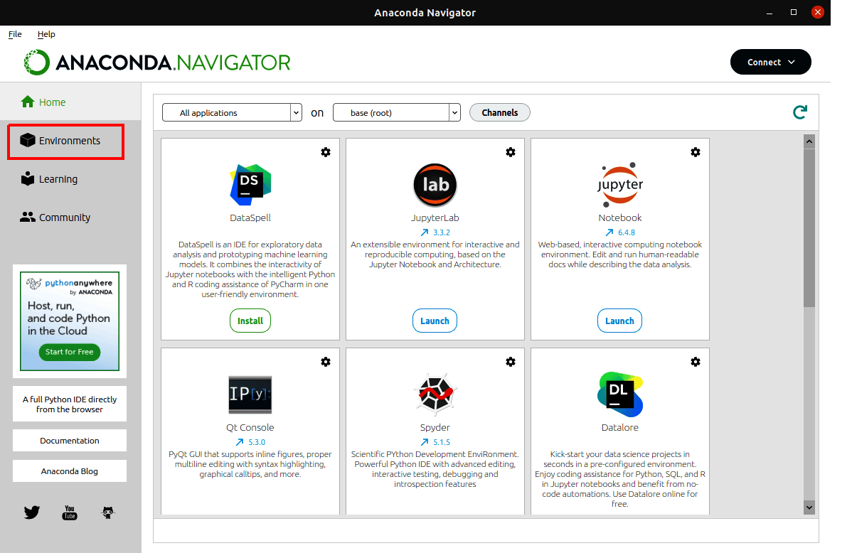
So, finally, we have reached a place in our journey where we no longer need to worry about installing the new packages and libraries necessary to continue our quest for developing AI and machine learning based applications. Notice that Anaconda only has a command-line interface (CLI). Are we in trouble? No! Our installation also gives us Anaconda Navigator, a graphical user interface (GUI) for Anaconda. Execute the command ‘anaconda-navigator’ on the terminal to run Anaconda Navigator (Figure 1). Soon, we will see an example of its power.
Introduction to Theano
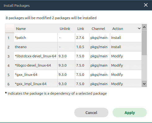
Now, let us try to work with Theano, a Python library and optimising compiler for evaluating mathematical expressions. The installation of Theano is very easy since we have Anaconda Navigator. First, open Anaconda Navigator. On the top right corner you will see the button Environments (marked with a red box in Figure 1). Press that button. You will go to a window showing the list of all currently installed packages. From the drop-down list on top, choose the option Not installed. Scroll down, find the option Theano, and click on the checkbox on the left. Now press the green button named Apply at the bottom right corner of the window. Anaconda will find out all the dependencies for installing Theano and show them in a pop-up menu. Figure 2 shows the pop-up menu I got during the installation of Theano in my system. You can see that in addition to Theano, one more new package is installed and eight other packages are modified.
Imagine how difficult this would have been if I was trying to manually install Theano. But with the help of Anaconda, all we need to do is press the button Apply on the bottom right corner of this pop-up menu. After a while, the installation of Theano will be completed smoothly. Now, we are ready to use Theano in our Jupyter Notebooks.
We are already familiar with the Python library called SymPy used for symbolic calculation but Theano takes it to the next level. Let us see a simple example to understand the power of Theano. Consider the code shown in Figure 3. First, let us try to understand the code. Line 1 of the code imports Theano. Line 2 imports tensor and names it T. We have already encountered tensors when we discussed TensorFlow.
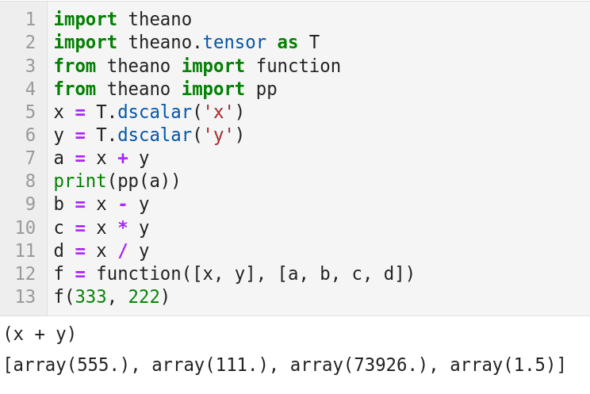
Mathematically, tensors can be treated as multi-dimensional arrays. Tensor is one of the key data structures used in Theano and can be used to store and manipulate scalars (numbers), vectors (1-dimensional arrays), matrices (2-dimensional arrays), tensors (multi-dimensional arrays), etc. In Line 3, a Theano function called function( ) is imported. Line 4 imports a Theano function called pp( ), which is used for pretty-printing (printing in a format appealing to humans). Line 5 creates a symbolic scalar variable of type double called x. It is a bit tricky to understand these sorts of symbolic variables. Think of it as a 0-sized double variable with no value or storage associated. Similarly, Line 6 creates another symbolic scalar variable called y. Line 7 acts like a function in a sense. This line tells the Python interpreter something like the following, ‘if and when symbolic scalar variables x and y get some values, add those values and store inside me’.
To further illustrate symbolic operations at this point, let us try to understand Line 8.
From Figure 3, it is clear that the output of this line of code is (x+y). So, it is clear that actual addition of two numbers is yet to take place. Lines 9 to 11 similarly define symbolic subtraction, multiplication, and division, respectively. If you want further clarity, use the function pp( ) to find the values of b, c, and d. Line 12 is very critical. It defines a function named f( ) using the function function( ) of Theano. The function function( ) takes two parameters. Parameter 1 is the data to be operated upon and parameter 2 is the function to be applied on the data given as parameter 1. Here, the data is the two symbolic scalar variables x and y. The function is given by [a b c d] which represents symbolic addition, subtraction, multiplication, and division, respectively. Finally, in Line 13, the function f( ) is provided with actual values rather than symbolic ones. The output of this operation is also shown in Figure 3. It is very easy to verify that the output shown is correct.
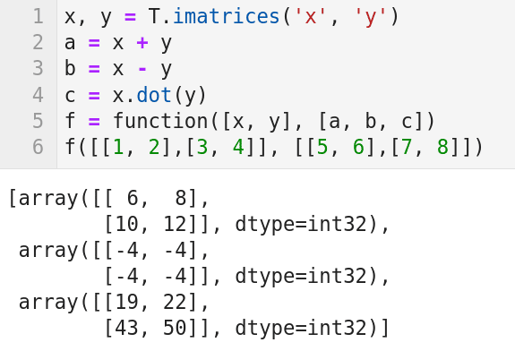
Now, let us see how matrices can be created and manipulated using Theano. Consider the code shown in Figure 4. It is important to note that the first three lines of code shown in Figure 3 should be added here also, if you are writing this program independent of the programs we have discussed so far. Now, let us try to understand the code. Line 1 of the code creates two symbolic matrices x and y. Think of x and y as two 0-dimensional arrays. But this time these matrices are of type integer unlike the last time where the data type was double. Further, this time a plural constructor (imatrices) is used so that more than one matrix can be constructed at the same time. Lines 3 to 5 perform symbolic addition, subtraction, and multiplication, respectively, on symbolic matrices x and y. Here again you can use print(pp(a)), print(pp(b)), and print(pp(c)) to better understand the symbolic nature of the operations being performed. If you add these lines of code, you will get (x+y), (x-y), and (x \dot y), respectively, as output. Line 5 generates a function f( ) which takes two parameters as before. Again, parameter 1 is the data to be operated upon and parameter 2 is the function to be applied on the data given as parameter 1. But this time, the data is the two symbolic matrices x and y. The function is given by [a b c] which represents symbolic addition, subtraction, and multiplication, respectively. Finally, in Line 6, the function f( ) is provided with actual values rather than symbolic ones. The two matrices given as input to f( ) are [[1, 2], [3, 4]] and [[5, 6], [7, 8]]. The output of this operation is also shown in Figure 4. It is very easy to verify that the three output matrices shown are correct. Notice that, in addition to scalars and matrices (for both of which we saw examples now), tensor also offers constructors like vector, row, column, different types of tensors, etc. Let us stop discussing Theano for now and revisit it while discussing advanced topics in probability and statistics.
Baby steps with probability
Now, let us continue discussing probability and statistics. I had suggested in the last article (while introducing probability) that you carefully go through three Wikipedia articles, and with that assumption of familiarity I tried to motivate you by discussing the Normal distribution. However, we must revisit some of the basic notions of probability and statistics before we start developing AI and machine learning based applications. I hope all of you have heard about arithmetic mean and standard deviation (SD).
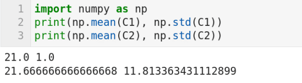
Arithmetic mean can be thought of as the average of a set of values. SD can be thought of as the variation or dispersion of a set of values. If the SD value is low then the elements in the set tend to be closer to the mean. On the contrary, if the SD value is high then the elements of the set are spread out over a wider range. But how can we calculate arithmetic mean and SD using Python? There is a module called statistics available with Python which can be used to find mean and standard deviation. However, experts are of the opinion that this module is very slow and hence we choose NumPy. Now, consider the code shown in Figure 5.
The code prints the mean and standard deviation of two lists C1 and C2 (whose values are hidden from you for the time being because of obvious reasons). What interpretations can you make from these values? Nothing! They are just numbers for you right now. But what if I tell you the lists contain the marks of six students, studying in 10th standard in school A and school B, for an exam in mathematics (the exam is out of 50 with a pass mark of 20). The mean value tells us that students from both the schools have relatively poor average marks with school B slightly outperforming school A. But what does the standard deviation value tell us? To further your understanding, I will give you the two lists, ‘C1 = [20, 22, 20, 22, 22, 20]’ and ‘C2 = [18, 16, 17, 16, 15, 48]’. Though hidden by the mean, the large standard deviation value of 11.813363431112899 clearly captures the mass failure in school B. This example clearly tells us that we need more complicated parameters to understand the complex nature of the problems we deal with. Probability and statistics will come to our rescue here by providing more and more complex models which can imitate complex and chaotic data.
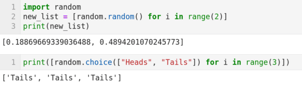
Random number generation is an essential part of probability. But, in practice, only pseudorandom number generation (a sequence of numbers whose properties approximate the properties of sequences of random numbers) is possible. Now, let us see a few functions that will help us generate pseudorandom numbers. Consider the code shown in Figure 6. First, let us try to understand the code. Line 1 imports the random package of Python. In Line 2, the function random.random( ) generates random numbers. This line of code, ‘new_list = [random.random() for i in range(2)]’, uses a technique called list comprehension to generate two random numbers and store them in the list named new_list. Line 3 prints this list as output. Notice that the two random numbers printed change with each iteration of the code, and the probability of getting the same numbers printed twice consecutively is theoretically zero. The single line of code in the second cell shown in Figure 6 uses the function random.choice( ). This function makes an equally likely choice from all the choices given to it. In this case, the code fragment random.choice([“Heads”, “Tails”]) will make a choice between ‘Heads’ or ‘Tails’ with equal probability. Notice that this line of code also uses the technique called list comprehension so that three successive choices between ‘Heads’ or ‘Tails’ are made. Figure 6 shows the output of this code, where the option ‘Tails’ is chosen for three consecutive times.
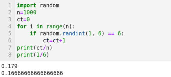
Now, let us try to illustrate a very popular theorem in probability, the law of large numbers (LLN), with a simple example. LLN states that the average of the results obtained from a large number of trials should be close to the expected value. Further, this average tends to come closer and closer to the expected value as more and more trials are performed. We all know that if a fair dice is thrown, the probability of getting the number 6 is 1/6. We now simulate this experiment with a simple Python code shown in Figure 7. Line 1 imports the random package of Python. Line 2 sets the number of trials to be performed. In this case, it is 1000. Line 3 initialises the counter ct to zero. Line 4 sets a loop, which iterates 1000 times in this case. Line 5 uses the function random.randint(1, 6). In this case, the function generates an integer between 1 and 6 (inclusive of both 1 and 6) randomly. The if statement in Line 5 checks whether the number generated is equal to 6; if yes the control goes to Line 7 and increases the counter ct by 1. After the loop is iterated a 1000 times, Line 8 will be executed. Line 8 prints the ratio between the number of occurrences of the number 6 and the total number of trials (1000). Figure 7 also shows this number as 0.179 (slightly more than the expected value 1/6 = 0.1666…which is also printed in the output). Not that close to the expected value, right? In Line 2, set the value of n as 10000. Run the code again and observe the new output printed. Most probably you will get a number which is a little bit closer to the expected value. Notice that this could also be a number less than the expected value. Increase the value of n, in Line 2, for a few more times. You will observe that the output is inching closer and closer to the expected value. Thus, with a simple code, we have illustrated LLN.
Though a simple statement, you will be amazed to know that the list of mathematicians who worked on a proof for LLN or tried to refine one include Cardano, Jacob Bernoulli, Daniel Bernoulli, Poisson, Chebyshev, Markov, Borel, Cantelli, Kolmogorov, Khinchin, etc. All of them are mathematical giants in their own field.
We are yet to cover topics in probability like random variables, probability distributions, etc, which are essential in developing AI and machine learning based applications. Our discussion of topics in probability and statistics is still in the early stages and we will try to strengthen our knowledge of these subjects in the next article also. At the same time, we will revisit two of our old friends we met in this journey earlier, the libraries Pandas and TensorFlow. We will also befriend a relative of TensorFlow called Keras, a library which acts as an interface for TensorFlow.


