


Natural language processing (NLP) helps computers understand and generate written and spoken words. NLP uses Term Frequency-Inverse Document Frequency to analyse the importance of a word within a document by assigning a numerical score to each word. Let’s find out how…
Term Frequency-Inverse Document Frequency (TF-IDF) is a method to convert text into numerical features. TF-IDF assigns higher weightages to important words in a corpus and reduces the importance of general words like ‘the’, ‘a’, ‘if’ by assigning lesser importance to them.
To establish the importance of a word, this approach first determines ‘how often the word appears in a document’; then it searches all the documents to determine ‘how rare the word is across all documents’. The first exercise is known as Term Frequency (TF) and the second is known as Inverse Document Frequency (IDF). The multiplication of these two parameters, i.e., TF x IDF, provides the weightage of that word. If a word is frequent in a specific document but rare across others, then the word is more important and gets a higher weightage.
This strategy helps us to remove the bias from frequently used uninformative words (e.g., ‘the’, ‘is’, ‘are’). It also identifies keywords of a document. This helps us to classify a document to identify its topic model by retrieving meaningful keywords from the target documents.
Simple example of TD-IDF
Assume we have three documents:
Doc1: “this magazine is great”
Doc2: “this magazine is bad”
Doc3: “The quality of this magazine is great”
Step 1: Vocabulary
Unique terms = {this, magazine, is, great, bad, quality, of}
| Term | Doc1 | Doc2 | Doc3 |
| this | low | low | low |
| magazine | high | high | high |
| is | low | low | low |
| great | high | 0 | high |
| bad | 0 | high | 0 |
| quality | 0 | 0 | high |
| of | 0 | 0 | high |
Weightage = {this: low, magazine: high, is: low, great: high, bad: high, quality: high, of: low}
| Term | Doc1 | Doc2 | Doc3 |
| this | 1 | 1 | 1 |
| magazine | 1 | 1 | 1 |
| is | 1 | 1 | 1 |
| great | 1 | 0 | 1 |
| bad | 0 | 1 | 0 |
| quality | 0 | 0 | 1 |
| of | 0 | 0 | 1 |
..
Words like ‘magazine’, ‘great’, ‘bad’, and ‘quality’ have higher TF-IDF weights because they are important in individual documents.
Step 2: Compute TF-IDF matrix
The components of TF-IDF are:
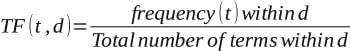
1. TF (Term Frequency): It measures the frequency of a term within a document.
2. IDF (Inverse Document Frequency): It measures the uniqueness of the words across the documents.
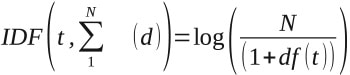
N = total number of documents
df(t) = number of documents containing the term ‘t’
3. TF-IDF score
Combining TF and IDF, the final TF-IDF formula is:
![]()
4. TF (Term Frequency) table
| Term | Doc1 (TF) | Doc2 (TF) | Doc3 (TF) |
| magazine | 1/4 | 1/4 | 1/7 |
| great | 1/4 | 0 | 1/7 |
| bad | 0 | 1/4 | 0 |
| quality | 0 | 0 | 1/7 |
5. IDF table
| Term | Appearance in documents | IDF |
| magazine | d1, d2, d3 | -0.12493874 |
| great | d1, d3 | 0 |
| bad | d2 | 0.176091259 |
| quality | d3 | 0.176091259 |
6. TF-IDF table
| Term | Doc1 | Doc2 | Doc3 |
| magazine | -0.03 | -0.03 | -0.02 |
| great | 0.00 | 0.00 | 0.03 |
| bad | 0.00 | 0.04 | 0.00 |
| quality | 0.00 | 0.00 | 0.03 |
‘great’ and ‘quality’ have higher TF-IDF values because they are rare and carry information for the classification of these documents. ‘magazine’ has negative IDF values and is therefore less useful for the classification of these sentiments.
Implementation
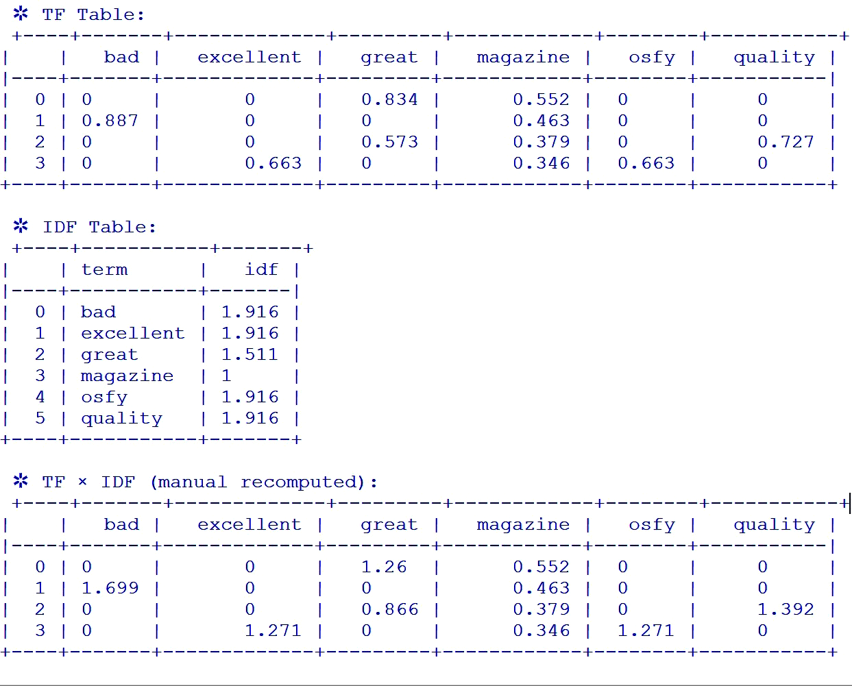
Here is a Python implementation of TD-IDF with four documents. The TF-IDF text processing technique can be easily understood by using this code, which generates TF, IDF, and TF x IDF tables. Scikit-learn is the most appropriate source for the TF-IDF library.
from sklearn.feature_extraction.text import TfidfVectorizer

from tabulate import tabulate

import pandas as pd

pd.set_option(‘display.max_columns’, None)

# Sample documents

corpus = [

“this magazine is great”, #Doc1

“this magazine is bad”, #Doc2

“the quality of this magazine is great”, #Doc3

“the name of this excellent magazine is OSFY”, #Doc4

]

# Create TF-IDF vectorizer object

vectorizer = TfidfVectorizer(stop_words=’english’, use_idf=True)

# Fit and transform the corpus

vector = vectorizer.fit_transform(corpus)

# Vocabulary

# TF

feature_names = vectorizer.get_feature_names_out()

df= pd.DataFrame(vector.toarray(), columns=feature_names)

# IDF TABLE

# Get IDF values for each term

idf_values = vectorizer.idf_

idf_df = pd.DataFrame({‘term’: feature_names, ‘idf’: idf_values})

# Multiply TF × IDF

tf_df = df

manual_tfidf = tf_df * idf_df.set_index(‘term’).T.loc[‘idf’]

manual_tfidf = manual_tfidf.round(3)

# Display all

print(“ \u2732 TF Table:\n”, tabulate(round(df,3), “keys”, tablefmt=”psql”))

print(“\n \u2732 IDF Table:\n”, tabulate(round(idf_df.round(3),3), “keys”, tablefmt=”psql”))

print(“\n \u2732 TF × IDF (manual recomputed):\n”, tabulate(round(manual_tfidf.round(3),3), “keys”, tablefmt=”psql”))
The TF-IDF values for each feature word in documents 0, 1, 2, and 3 are displayed in the final TD-IDF table. While a frequent feature word (magazine) has lower scores and is therefore less significant, feature words with a rare appearance have higher TF-IDF values. These documents’ key terms include ‘bad’, ‘excellent’, ‘great’, ‘osfy’, and ‘quality’.
N-grams
The idea of n-grams is widely used in a variety of NLP applications, such as text prediction, information retrieval, and language modelling, where capturing the statistical characteristics of text becomes essential to understand the functionality of the underlying model. A contiguous sequence of ‘n’ items from a given text or speech is known as an n-gram in natural language processing. The object may be a word, syllable, character, etc. A ‘unigram’ is an n-gram of size 1, a ‘bigram’ is a size 2, and a ‘trigram’ is a size 3.
TF-IDF vectorization uses n-gram with an ngram_range parameter, which is a tuple (min_n, max_n). Min_n and max_n establish the lower and upper bounds of the n-gram sizes, allowing n-grams to be explored within this range. For example, if ngram_range is set to (1, 3), the ‘vectorizer’ will extract unigrams, bigrams, and trigrams, adding a wider context to the feature set used for machine learning models.
Selecting an appropriate n-gram range can have a considerable impact on the analysis of NLP tasks. Unigrams, for example, may not successfully convey context (e.g., ‘not excellent’ versus just ‘excellent’), whereas bigrams, trigrams, or even higher-level n-grams may.
Unigram TF-IDF
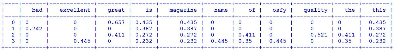
The sklearn package makes summarising a corpus an easy task. The following code is an illustration of unigram analysis.
from sklearn.feature_extraction.text import TfidfVectorizer
from tabulate import tabulate
import pandas as pd
# Sample documents
corpus = [
“this magazine is great”, #Doc1
“this magazine is bad”, #Doc2
“the quality of this magazine is great”, #Doc3
“the name of this excellent magazine is OSFY” #Doc4
]
# Create TF-IDF vectorizer object
vectorizer = TfidfVectorizer()
# Fit and transform the corpus
vector = vectorizer.fit_transform(corpus)
# Convert to array and print
#print(vector.toarray())
# Vocabulary
feature_names = vectorizer.get_feature_names_out()
df= pd.DataFrame(vector.toarray(), columns=feature_names)
print(round(df,3))
Bigram TF-IDF
Here is an example with the same corpus using bigram.
# Create TF-IDF vectorizer object
vectorizer = TfidfVectorizer(
max_features=500,
stop_words=’english’,
ngram_range=(2,2), # bigrams
min_df=1, # ignore rare words
max_df=0.85 # ignore too frequent words
)
# Fit and transform the corpus
vector = vectorizer.fit_transform(corpus)
vector_df = pd.DataFrame(vector.toarray())
# Vocabulary
feature_names= vectorizer.get_feature_names_out()
#print(feature_names)
#print(tabulate(vector_df, headers=feature_names, tablefmt=”grid”))
# Convert to array and print
df= pd.DataFrame(vector.toarray(), columns=feature_names)
print(round(df,3))
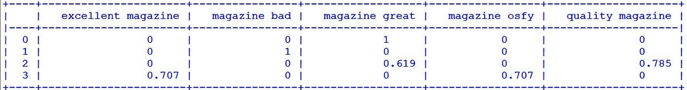
Bigram gives us four meaningful contextual phrases, such as ‘quality magazine’, ‘excellent magazine’, ‘bad magazine’, and ‘osfy magazine’, together with the matching TF-IDF values for each of the four documents. These four bigrams also serve as indicative keywords for the corpus and point to OSFY magazine as a high-quality publication.


