































































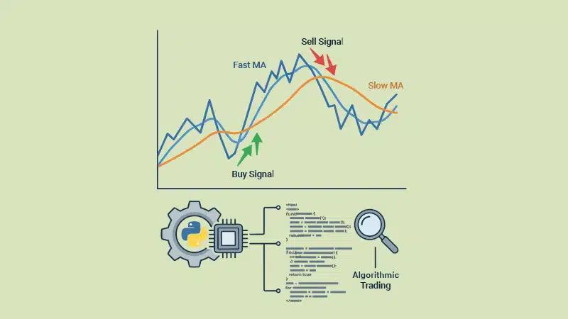

Traders on the stock market can take advantage of the Moving Average Crossover Strategy to maximise the returns on their investments.
The Moving Average Crossover Strategy is probably the easiest and most effective trading algorithm that can help teach algorithmic trading. It uses only the price history of a stock and several lines of Python to cover nearly all the concepts used when designing a trading Python script strategy: market data, technical indicators, trading signals, positions, profits, risks, transaction costs, and performance. The main idea behind this strategy is to make use of the correlation between short-term and long-term moving averages to determine changes in market trends.
What is a moving average?
The moving average smoothens out the fluctuations in the prices of a stock by calculating the average price for ‘n’ periods preceding the current one. The formula used to compute the SMA (simple moving average) is:

…where Pt represents the closing price at time ‘t’. For example, if the closing prices for five days are:
|
Day 1 |
100 |
|
Day 2 |
102 |
|
Day 3 |
101 |
|
Day 4 |
105 |
|
Day 5 |
107 |
…the 5-day moving average is:

With each new price, the old data point is dropped, and the new data point is added. This process can be carried out quite easily in Python using the Pandas’ rolling function; a 20-day moving average will be computed as follows:
df[“SMA20”] = df[“Close”].rolling(20).mean()
…where ‘df’ is a historical market DataFrame.
Why use two moving averages?
A single moving average tells us about the general direction of the market, but two moving averages allow us to identify the changes in a trend. For example, if we consider 20 days and 50 days for short-term and long-term moving averages, the 20-day moving average will react relatively quickly to changes in price, while the 50-day moving average will change more slowly. The relationship between them gives us a simple trading rule:
20-day SMA > 50-day SMA → Bullish → Hold
…and:
20-day SMA < 50-day SMA → Bearish → Exit
The actual crossing of the two averages is called a crossover.
Golden Cross and Death Cross
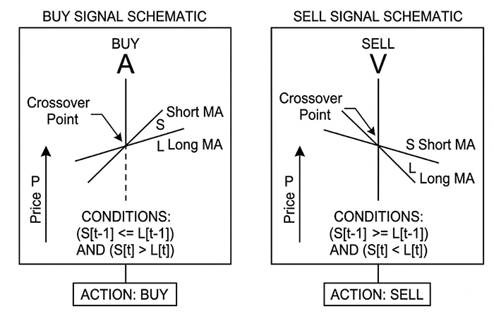
Two popular names for the Moving Average Crossover Strategy are Golden Cross and Death Cross. When the shorter MA crosses above the longer MA the situations are known as Golden Crosses and are usually seen as a positive signal. On the other hand, when the shorter MA crosses below the longer MA the incidents known as Death Crosses and are usually seen as a negative signal.
The periods used in the calculation of the moving average are not always the same and can range from 5/20 and 10/30, to 20/50 and 50/200.
The crossover between the short-term and long-term moving averages helps us to determine the positioning strategy for trading. This has been summarised in Figure 1.
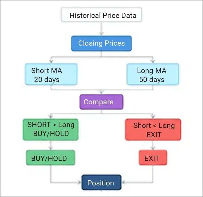
This simple workflow forms the basis of our Python implementation.
Obtaining market data with Python
For a study, historical market data can be obtained using yfinance.
import yfinance as yf

import pandas as pd

import matplotlib.pyplot as plt

ticker = “TCS.NS”

df = yf.download(

ticker,

start=”2020-01-01”,

end=”2025-01-01”,

auto_adjust=True,

progress=False,

threads=False

)
| print(df.head())Close | High | Low | Open | Volume |
| TCS.NS | TCS.NS | TCS.NS | TCS.NS | TCS.NS |
| 1831.11 | 1844.879 | 1819.621 | 1831.447 | 1354908 |
| 1822.704 | 1841.543 | 1815.566 | 1841.543 | 2380752 |
| 1859.029 | 1877.91 | 1828.069 | 1828.069 | 4655761 |
| 1858.86 | 1880.401 | 1848.258 | 1862.703 | 3023209 |
| 1863.422 | 1870.856 | 1844.795 | 1858.903 | 2429317 |
Before proceeding further, always check that the download was successful:
if df.empty:

raise ValueError(“No market data was downloaded.”)
The resulting DataFrame may have MultiIndex columns depending upon the yfinance package version. In case it’s needed, get the data for a single ticker/attribute using the xs() method.
if isinstance(df.columns, pd.MultiIndex):

df = df.xs(ticker, axis=1, level=”Ticker”)
Then remove all null recordsets:
df = df.dropna()
Calculating the moving averages
We now calculate the short and long moving averages for two moving window sizes — 20 and 50:
short_window = 20

long_window = 50

df[“SMA20”] = (

df[“Close”]

.rolling(short_window)

.mean()

)

df[“SMA50”] = (

df[“Close”]

.rolling(long_window)

.mean()

)

print(

df[

[“Close”, “SMA20”, “SMA50”]

].tail()

}
Close |
SMA20 | SMA50 |
| 3892.482 | 4042.155 | 3910.172 |
| 3882.796 | 4034.544 | 3910.964 |
| 3878.838 | 4030.816 | 3912.046 |
| 3873.203 | 4025.599 | 3913.421 |
| 3813.598 | 4017.13 | 3913.343 |
Plotting the moving averages
Though browsing the record set with a short- and long-term moving average shows new feature columns, visualisation plays a special role in understanding the price movement pattern.
plt.figure(figsize=(15, 7))

plt.plot(

df.index,

df[“Close”],

label=”Close Price”,

linewidth=1.2

)

plt.plot(

df.index,

df[“SMA20”],

label=”20-Day SMA”,

linewidth=2

)

plt.plot(

df.index,

df[“SMA50”],

label=”50-Day SMA”,

linewidth=2

)

plt.title(

f”{ticker} — Moving Average Crossover”

)


plt.xlabel(“Date”)

plt.ylabel(“Price”)

plt.legend()

plt.grid(True, alpha=0.3)

plt.tight_layout()

plt.show()
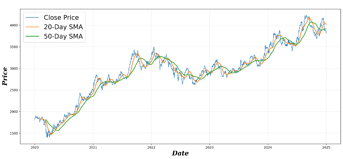
To study the crossover, it’s important to look for the points at which the short-term average crosses the long-term average (Figure 2).
Detecting Buy and Sell crossover points
The critical difference lies in whether the price is above/below the long-term moving average or crosses the moving average.
A Buy crossover occurs when:
Yesterday: SMA20 <= SMA50
Today: SMA20 > SMA50
In Python this can be implemented as:
buy = (

(df[“SMA20”] > df[“SMA50”]) &

(df[“SMA20”].shift(1) <= df[“SMA50”].shift(1))

)
Similarly, a Sell crossover occurs when:
Yesterday: SMA20 >= SMA50
Today: SMA20 < SMA50
This can be implemented as:
sell = (

(df[“SMA20”] < df[“SMA50”]) &

(df[“SMA20”].shift(1) >= df[“SMA50”].shift(1))

)
The shift(1) is important because it allows us to compare today’s relationship with yesterday’s relationship.
Creating the trading position
We now convert the moving average relationship into a position by identifying the Buy/Sell signals:
Thus:
Signal = 1 → Holding the stock

Signal = 0 → Not holding the stock
We can visualise the position:
print(

df[

[“Close”, “SMA20”, “SMA50”, “Signal”]

].tail(20)

)
Close |
SMA20 | SMA50 | Signal |
| 4007.268 | 3890.032 | 3879.731 | 1 |
| 4055.371 | 3908.205 | 3881.22 | 1 |
| 4157.49 | 3931.148 | 3885.056 | 1 |
| 4140.215 | 3945.39 | 3888.494 | 1 |
| 4146.408 | 3959.419 | 3891.992 | 1 |
Marking all crossovers on the chart
After knowing the position indicator, it is possible to integrate the price, the moving averages, the Buy indicators, and the Sell indicators into a visual report on the entire trading process.
fig, ax = plt.subplots(figsize=(15, 7))

ax.plot(

df.index,

df[“Close”],

label=”Close Price”,

linewidth=1.2

)

ax.plot(

df.index,

df[“SMA20”],

label=”20-Day SMA”,

linewidth=2

)

ax.plot(

df.index,

df[“SMA50”],

label=”50-Day SMA”,

linewidth=2

)

# BUY signals

ax.scatter(

df.index[buy],

df.loc[buy, “Close”],

marker=”^”,

s=120,

label=”BUY”,

zorder=5

)

# SELL signals

ax.scatter(

df.index[sell],

df.loc[sell, “Close”],

marker=”v”,

s=120,

label=”SELL”,

zorder=5

)

ax.set_title(

f”{ticker} — 20/50 Moving Average Crossover”

)

ax.set_xlabel(“Date”)

ax.set_ylabel(“Price”)

ax.legend()

ax.grid(True, alpha=0.3)

plt.tight_layout()

plt.show()
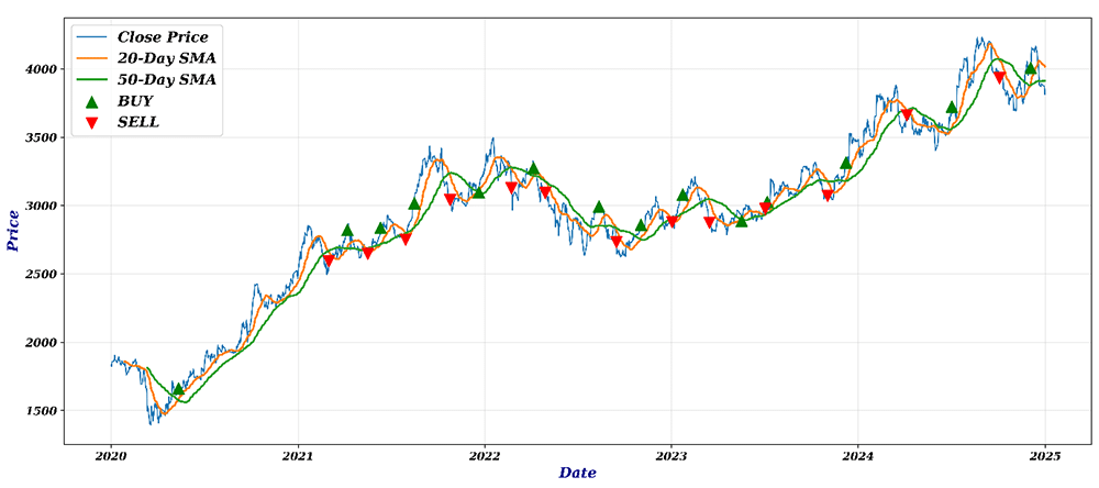
The chart now provides a visual representation of the positioning algorithm (Figure 3).
How the strategy helps to hold stock
Finally, for a clear demonstration of the Hold and Sell periods along the entire moving average cycle we can shade the holding periods of the stock. This is particularly useful for understanding the trading pattern.
holding = df[“Signal”] == 1
The shading of the periods during which the strategy helps to hold the stock is implemented here and shown in Figure 5:
fig, ax = plt.subplots(figsize=(15, 7))

ax.plot(

df.index,

df[“Close”],

label=”Close Price”,

linewidth=1.2

)

ax.plot(

df.index,

df[“SMA20”],

label=”20-Day SMA”,

linewidth=2

)

ax.plot(

df.index,

df[“SMA50”],

label=”50-Day SMA”,

linewidth=2

)

# Holding periods

ax.fill_between(

df.index,

0,

1,

where=holding,

transform=ax.get_xaxis_transform(),

alpha=0.12,

label=”Holding Position”

)

# BUY

ax.scatter(

df.index[buy],

df.loc[buy, “Close”],

marker=”^”,

s=120,

label=”BUY”,

zorder=5

)

# SELL

ax.scatter(

df.index[sell],

df.loc[sell, “Close”],

marker=”v”,

s=120,

label=”SELL”,

zorder=5

)

ax.set_title(

f”{ticker} — Moving Average Crossover Strategy”

)

ax.set_xlabel(“Date”)

ax.set_ylabel(“Price”)

ax.legend()

ax.grid(True, alpha=0.3)

plt.tight_layout()

plt.show()
Buy zone: In Figure 5, when the short moving average crosses over the long moving average, the stock should be bought.
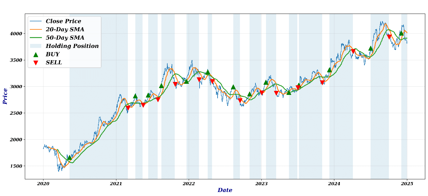
Hold zone: When the short moving average stays over the long moving average, the stock should be held.
Sell zone: When the short moving average crosses under the long moving average, the stock should be sold.
This provides traders with a direct visual relationship between the crossover and the position, and between the position and the holding period.
Traders can optimise the entire process of SMA crossover through backtesting using different time periods of moving averages — for example, 5/10, 10/30, and 50/200. However, algorithmic trading is not just about producing Buy and Sell signals. It needs much more than that to build a robust strategy.